Density based clustering basics

Go to:

• Notebook configuration

• Helper function definitions

• Density criteria

• Identification of connected components

• CommonNN clustering in detail

Notebook configuration

from collections import deque
from itertools import islice
import sys

import matplotlib as mpl
from matplotlib import animation
import matplotlib.pyplot as plt
import networkx
import numpy as np
import scipy
from scipy.integrate import quad
from scipy import stats
from scipy.spatial import cKDTree
import sklearn
from sklearn import datasets
from sklearn.preprocessing import StandardScaler

import cnnclustering
from cnnclustering import cluster
from cnnclustering import _types, _fit

Print Python and package version information:

# Version information
print("Python: ", *sys.version.split("\n"))

print("Packages:")
for package in [mpl, networkx, np, scipy, sklearn, cnnclustering]:
    print(f"    {package.__name__}: {package.__version__}")

Python:  3.8.8 (default, Mar 11 2021, 08:58:19)  [GCC 8.3.0]
Packages:
    matplotlib: 3.3.4
    networkx: 2.5
    numpy: 1.20.1
    scipy: 1.6.1
    sklearn: 0.24.1
    cnnclustering: 0.4.3

We use Matplotlib to create plots. The matplotlibrc file in the root directory of the CommonNNClustering repository is used to customize the appearance of the plots.

# Matplotlib configuration
mpl.rc_file(
    "../../matplotlibrc",
    use_default_template=False
)

Helper function definitions

The following functions will be used throughout this notebook.

def gauss(x, sigma, mu):
    """Gaussian PDF"""
    return (1 / (sigma * np.sqrt(2 * np.pi)) * np.exp(-1 / 2 * ((x - mu) / sigma)**2))

def multigauss(x, sigmas, mus):
    """Multimodal gaussian PDF as linear combination of gaussian PDFs"""
    assert len(sigmas) == len(mus)

    out = np.zeros_like(x)
    for s, m in zip(sigmas, mus):
        out += gauss(x, s, m)
    return out / len(sigmas)

def determine_cuts(x, a, cutoff):
    """Find points in 1D space where density cutoff is crossed

    Args:
       x: coordinate
       a: density
       cutoff: density cutoff

    Returns:
       cuts: Array of coordinates where cutoff is crossed
    """

    cuts = []
    dense = False  # Assume low density on left border
    for index, value in enumerate(a[1:], 1):
        if dense:
            if value < cutoff:
                dense = False
                cuts.append((x[index] + x[index - 1]) / 2)
        else:
            if value >= cutoff:
                dense = True
                cuts.append((x[index] + x[index - 1]) / 2)

    return np.asarray(cuts)

class multigauss_distribution(stats.rv_continuous):
    """Draw samples from a multimodal gaussian distribution"""

    def __init__(self, sigmas, mus, *args, **kwargs):
        super().__init__(*args, **kwargs)
        self._sigmas = sigmas
        self._mus = mus

    def _pdf(self, x):
        return multigauss(x, sigmas=self._sigmas, mus=self._mus)

Density criteria

Density-based clustering defines clusters as dense regions in space, separated by sparse regions. But what is dense and what is sparse? This is commonly defined by a threshold (a density criterion) that determines the outcome of the clustering. In the case where we have a density function defined on a continuous coordinate, the density criterion manifests itself as a density iso-surface. Regions in which the density is higher than a cutoff set as density criterion qualify as dense, and therefore represent a cluster. On the other hand, regions in which the density falls below the density criterion are considered sparse and do not constitute a part of a cluster. We can illustrate this on the example of a bimodal gaussian distribution in one dimension.

xlimit = (-8, 8)
x = np.linspace(*xlimit, 101)

fig, ax = plt.subplots()
ax.plot(x, multigauss(x, sigmas=[1, 1.5], mus=[-2, 2]))
ax.set(**{
    "xlim": xlimit,
    "xlabel": "$x$",
    "ylabel": "probability density"
})
plt.show()

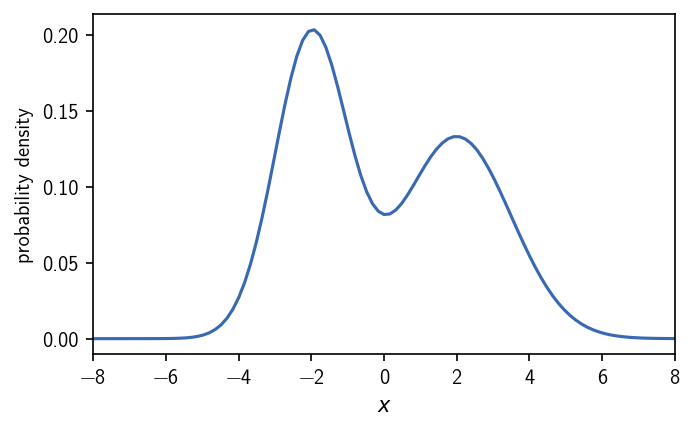
We have two maxima in the distribution. An intuitive classification would separate the two peaks into two different clusters. In threshold-based density based clustering we define the two clusters as the regions of high density where we have low density in between. By applying an iso-value cutoff on the density, we can specify what should be considered high or low density. In a dense region, the density is at least as high as the density criterion requires.

density_criterion = 0.1

xlimit = (-8, 8)
x = np.linspace(*xlimit, 1001)
pdf = multigauss(x, sigmas=[1, 1.5], mus=[-2, 2])
cuts = determine_cuts(x, pdf, density_criterion)
density_criterion_ = np.full_like(x, density_criterion)
dense = np.maximum(pdf, density_criterion_)

fig, ax = plt.subplots()
ax.plot(x, pdf)
ax.plot(x, density_criterion_, linestyle="--", color="k")
ax.fill_between(x, density_criterion_, dense)
for cut in cuts:
    ax.axvline(cut, color="gray", alpha=0.5)

ax.annotate(
    "density criterion", (xlimit[0] * 0.975, density_criterion * 1.03),
    fontsize="small"
)

ax.annotate("0", (cuts[0] * 1.2, 0))
ax.annotate("1", (cuts[1] * 2, 0))
ax.annotate("0", (cuts[2] * 0.2, 0))
ax.annotate("2", (cuts[3] * 0.8, 0))
ax.annotate("0", (cuts[3] * 1.2, 0))

ax.annotate(
    "dense",
    xy=(2.2, multigauss(2.2, sigmas=[1, 1.5], mus=[-2, 2])),
    xytext=(cuts[3] * 1.2, density_criterion * 1.5),
    arrowprops={"arrowstyle": "->"}
)

ax.annotate(
    "sparse",
    xy=(4, multigauss(4., sigmas=[1, 1.5], mus=[-2, 2])),
    xytext=(cuts[3] * 1.2, density_criterion * 1.2),
    arrowprops={"arrowstyle": "->"}
)

ax.set(**{
    "xlim": xlimit,
    "xlabel": "$x$",
    "ylabel": "probability density"
})
plt.show()

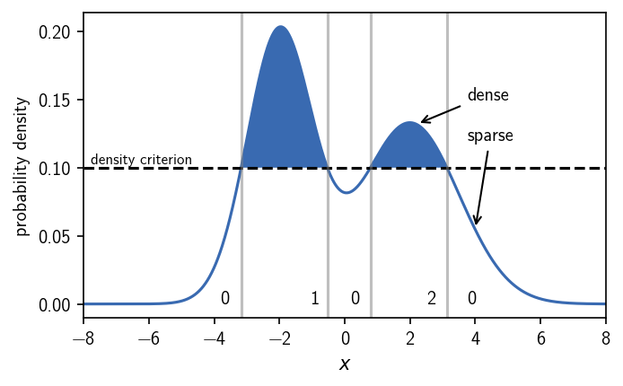
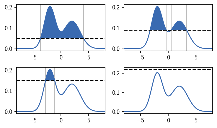
Choosing the density criterion in this way, defines the two clusters as we would have expected. We can label the regions, i.e. we can assign a number to them, that denotes their cluster membership. We use 0 to indicate that a region is not part of any cluster and positive integers as cluster numbers. When we vary the density criterion, we can influence the outcome of the clustering by changing the definition of what is dense enough to be a cluster. This could leave us with both density maxima in one cluster, clusters of different broadness, or no cluster at all.

fig, Ax = plt.subplots(2, 2)
ax = Ax.flatten()

for i, d in enumerate([0.05, 0.09, 0.15, 0.22]):
    density_criterion = d

    xlimit = (-8, 8)
    x = np.linspace(*xlimit, 1001)
    pdf = multigauss(x, sigmas=[1, 1.5], mus=[-2, 2])
    cuts = determine_cuts(x, pdf, density_criterion)
    density_criterion_ = np.full_like(x, density_criterion)
    dense = np.maximum(pdf, density_criterion_)


    ax[i].plot(x, pdf)
    ax[i].plot(x, density_criterion_, linestyle="--", color="k")
    ax[i].fill_between(x, density_criterion_, dense)
    for cut in cuts:
        ax[i].axvline(
            cut,
            color="gray",
            alpha=0.5,
            linewidth=1,
            zorder=0
            )


    ax[i].set(**{
        "xlim": xlimit,
    })

fig.tight_layout()
plt.show()

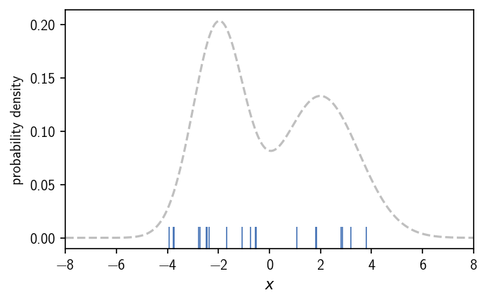
When we operate on data sets (in maybe high dimensional spaces), however, we normally do not have a continuous description of the density that we can directly use. Instead we may have sample points from an underlying (unknown) distribution. To apply a density based clustering on them, we need to approximate the density in some way. For this approximation, a number of different possibilities exist, which provide a different notion of what density is or how it could be estimated from scattered data. To illustrate this, let’s draw samples from the above used bimodal distribution to emulate data points.

distribution = multigauss_distribution(
    sigmas=[1, 1.5], mus=[-2, 2], a=-8, b=8, seed=11
)
samples = distribution.rvs(size=20)

xlimit = (-8, 8)
x = np.linspace(*xlimit, 1001)
pdf = multigauss(x, sigmas=[1, 1.5], mus=[-2, 2])

fig, ax = plt.subplots()
ax.plot(x, pdf, color="gray", linestyle="--", alpha=0.5)

ax.set(**{
    "xlim": xlimit,
    "xlabel": "$x$",
    "ylabel": "probability density"
})

ax.plot(samples, np.zeros_like(samples), linestyle="",
        marker="|", markeredgewidth=0.75, markersize=15)

plt.show()

In the following we look into how density is deduced from points in terms of the following methods:

• DBSCAN

• Jarvis-Patrick

• CommonNN

In general, point density can be expressed in simple terms by the number of points \(n\) found on a volume \(V\).

DBSCAN

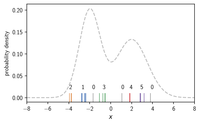
In DBSCAN, local point density is expressed for each point as the number of neighbouring points \(k_r\) with respect to a neighbour search radius \(r\). The density criterion is formulated as such: Points that have at least \(k\) nearest neighbours in their neighbourhood \(r\) qualify as part of a dense region, i.e. a cluster. Points that fulfill the density criterion can be also referred to as core points. Additionally it is possible to describe points that do not fulfill the density criterion themselves but are neighbours of those core points as edge points. For our samples above this could look as shown below if we choose the density criterion to be \(k=1\) and \(r=0.5\). To determine the number of neighbours for each point, we calculated pairwise point distances and compare them to \(r\).

# Density criterion
r = 0.5  # Neighbour search radius
k = 1    # Minimum number of neighbours

n_neighbours = np.array([
    # Neighbour within r?
    len(np.where((0 < x) & (x <= r))[0])
    # distance matrix
    for x in np.absolute(np.subtract.outer(samples, samples))
])

dense = n_neighbours >= k  # Point is part of dense region?
dense

array([ True,  True,  True,  True,  True,  True,  True,  True, False,
        True,  True,  True,  True,  True,  True, False,  True,  True,
       False,  True])

xlimit = (-8, 8)
x = np.linspace(*xlimit, 1001)
pdf = multigauss(x, sigmas=[1, 1.5], mus=[-2, 2])

fig, ax = plt.subplots()
ax.plot(x, pdf, color="gray", linestyle="--", alpha=0.5)

ax.set(**{
    "xlim": xlimit,
    "xlabel": "$x$",
    "ylabel": "probability density"
})

for i, s in enumerate(samples):
    if dense[i]:
        c = "#396ab1"
    else:
        c = "gray"
    ax.plot(s, 0, linestyle="",
            marker="|", markeredgewidth=0.75, markersize=15,
            color=c)

labels = [
    (-4, "1"),
    (-2.8, "2"),
    (-1.8, "0"),
    (-0.8, "3"),
    (1, "0"),
    (1.8, "4"),
    (2.8, "5"),
    (3.8, "0"),
]

for position, l in labels:
    ax.annotate(l, (position, 0.02))

plt.show()

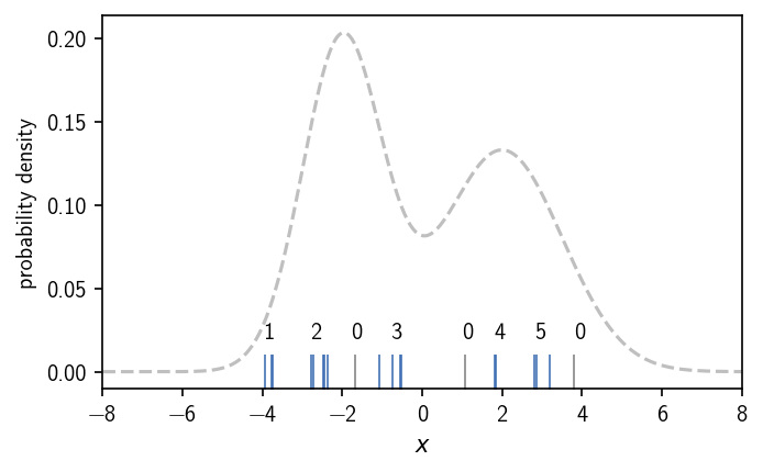
In this case we end up with 5 clusters, that are dense enough regions separated by low density areas. Like a change in the density iso-value as the density criterion for the continuous density function, a change of the cluster parameters \(k\) and \(r\) will determine the cluster result. Note, that we assigned the labels to the clusters by visual inspection. We will show later how to identify these isolated regions (connected components of core points) automatically. For this we additionally need to define when two points are actually part of the same dense region, meaning we need to define connectivity between points. In the case of DBSCAN, checking the density-criterion and checking the connectivity of two points are basically two separate tasks.

Common-nearest-neighbours clustering

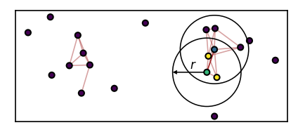
While the DBSCAN approach to threshold-based density-based clustering estimates point density locally per point, we determine the density between two points in CommonNN clustering. As a consequence, checking the density-criterion and defining if two points are connected become essentially the same thing. Two points that fulfill the density requirement together are automatically identified as part of the same cluster. The density threshold (points per volume) is formulated as such: Two points that share a minimum number of c common neighbours with respect to a neighbour search radius r are considered dense. The figure below illustrates this. The green and the blue point pass the density-criterion check for CommonNN cutoffs of \(c\leq2\) because they share the two yellow points as their common neighbours.

# samples2D = np.vstack([np.random.normal((-1, 0), (0.4, 0.4), (10, 2)), np.random.normal((1, 0), (0.4, 0.4), (10, 2))])
samples2D = np.load("algorithm_explained/samples2D.npy")

# Density criterion / density reachability in 2D
fig, ax = plt.subplots(figsize=(3.33, 2.05))
r = 0.5
c = 2

neighbourhoods = np.array([
    # Neighbour within r?
    np.where((0 < x) & (x <= r))[0]
    # distance matrix
    for x in np.sqrt(np.subtract.outer(samples2D[:, 0], samples2D[:, 0])**2 + np.subtract.outer(samples2D[:, 1], samples2D[:, 1])**2)
    ], dtype=object)

for node, neighbours in enumerate(neighbourhoods):
    for other_node in neighbours:
        if np.intersect1d(neighbours, neighbourhoods[other_node]).shape[0] >= c:
            # Density criterion fullfilled
            ax.plot(*zip(samples2D[node], samples2D[other_node]), color="brown", alpha=0.25, linewidth=0.75, zorder=0)

source = 12
member = 15
intersection = [13, 18]
classification = np.zeros(samples2D.shape[0])
classification[source] = 1
classification[member] = 2
classification[intersection] = 3

ax.plot(*zip(samples2D[source], samples2D[member]), color="brown", alpha=1, linewidth=0.75, zorder=0)

ax.annotate(
    "", (samples2D[member][0] - r, samples2D[member][1]), samples2D[member],
    arrowprops={
        "shrink": 0, "width": 0.75, "headwidth": 3, "headlength": 3,
        "facecolor": "k", "linewidth": 0
        },
    zorder=0
    )

ax.annotate(
    "$r$", (samples2D[member][0] - r/2, samples2D[member][1] + 0.05),
    fontsize=8
    )

ax.scatter(*samples2D.T, s=15, c=classification, linewidth=1, edgecolor="k")
neighbourhood = mpl.patches.Circle(
    samples2D[source], r,
    facecolor="None",
    edgecolor="k", linewidth=0.75
    )
neighbourhood2 = mpl.patches.Circle(
    samples2D[member], r,
    facecolor="None",
    edgecolor="k", linewidth=0.75
    )
ax.add_patch(neighbourhood)
ax.add_patch(neighbourhood2)
ax.set(**{
    "xticks": (),
    "yticks": (),
    "aspect": "equal"
})

[[], [], None]

How the density criterion check and the clustering could be implemented should be explained further down.

Summary on density criteria

A point is part of a dense region if the point …

• DBSCAN: … has at least \(k_r\) neighbours within a radius \(r\)

• Jarvis-Patrick: … shares at least \(c\) common neighbours with a another point among their \(k\) nearest neighbours

• CommonNN: … shares at least \(c\) common neighbours with a another point with respect to a radius \(r\)

Two points are part of the same dense region … - DBSCAN: … if at least one of them is dense and the two points are neighbours - Jarvis-Patrick: … if they together pass the density criterion - CommonNN: … if they together pass the density criterion

Identification of connected components of points

Classifying points as part of a dense or a sparse region according to a density criterion, is only one aspect of assigning points to clusters. We still need to identify groups of points that are part of the same region. In this context, the term density reachable is often used to describe the situation where a point is directly connected to a dense point. We also use the term density connected for points that are part of the same dense region, i.e. they are directly or indirectly connected to any other point in the region by a chain of density reachable points. In other words, it is not enough to know which points are dense but we also need to be aware of the relationship between dense points. As mentioned earlier, for CommonNN clustering density reachability is a direct consequence of how the density-criterion is checked. For DBSCAN, this is a separate definition.

When we express the connectivity relationship between points in a graph, the problem of identifying clusters of density connected points comes down to finding connected components of nodes within this graph. In the above example, we where primarily interested in the information if a point was part of a dense region by checking the density criterion. Let’s now construct a density graph instead in which each dense point constitutes a node and each vertex represent the density reachability between two points. We neglect the concept of edge points (points that are not dense but density reachable from a dense point) for the sake of simplicity here. It should be noted, that the inclusion of edge points may also lead to ambiguous clustering results in the case where a low density point is a neighbour of two or more dense points in different clusters.

DBSCAN

# Density criterion
r = 0.5  # Neighbour search radius
k = 1    # Minimum number of neighbours

neighbourhoods = [
    # Neighbour within r?
    np.where((0 < x) & (x <= r))[0]
    # distance matrix
    for x in np.absolute(np.subtract.outer(samples, samples))
]

n_neighbours = np.asarray([len(x) for x in neighbourhoods])
dense = n_neighbours >= k

# Construct graph as dictionary
# keys: dense points, values: density reachable points
graph = {}
for i, point in enumerate(neighbourhoods):
    if dense[i]:
        graph[i] = neighbourhoods[i][dense[neighbourhoods[i]]]

G = networkx.Graph(graph)
pos = networkx.spring_layout(G, iterations=10, seed=7)
networkx.draw(G, pos=pos)
plt.show()

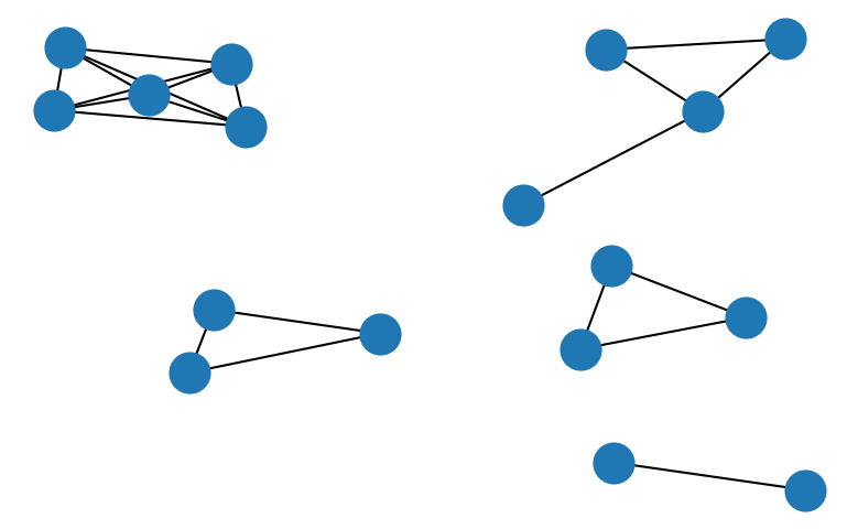
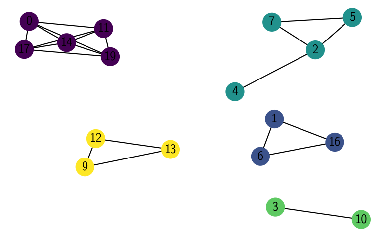
Once such a graph is constructed, graph traversal algorithms can be used to find the connected components of nodes within the graph. A generic way to do so using a breadth-first-search algorithm could look like this:

labels = {}                          # Cluster label assignments
visited = {k: False for k in graph}  # Node has been assigned
queue = deque()                      # First-in-first-out queue
current = 1                          # Current cluster number

for point, connected in graph.items():
    # Source node
    if visited[point]:
        continue

    labels[point] = current
    visited[point] = True

    while True:
        for reachable in connected:
            if visited[reachable]:
                continue

            labels[reachable] = current
            visited[reachable] = True
            queue.append(reachable)

        if not queue:
            break

        point = queue.popleft()
        connected = graph[point]

    current += 1

labels

{0: 1,
 11: 1,
 14: 1,
 17: 1,
 19: 1,
 1: 2,
 6: 2,
 16: 2,
 2: 3,
 4: 3,
 5: 3,
 7: 3,
 3: 4,
 10: 4,
 9: 5,
 12: 5,
 13: 5}

networkx.draw(G, pos=pos, with_labels=True, node_color=[x[1] for x in sorted(labels.items())])
plt.show()

xlimit = (-8, 8)
x = np.linspace(*xlimit, 1001)
pdf = multigauss(x, sigmas=[1, 1.5], mus=[-2, 2])

fig, ax = plt.subplots()
ax.plot(x, pdf, color="gray", linestyle="--", alpha=0.5)

ax.set(**{
    "xlim": xlimit,
    "xlabel": "$x$",
    "ylabel": "probability density"
})

colors = ['#396ab1', '#da7c30', '#3e9651', '#cc2529', '#6b4c9a']
for i, s in enumerate(samples):
    if dense[i]:
        c = colors[labels[i] - 1]
    else:
        c = "gray"
    ax.plot(s, 0, linestyle="",
            marker="|", markeredgewidth=0.75, markersize=15,
            color=c)

labels_ = [
    (-4, "2"),
    (-2.8, "1"),
    (-1.8, "0"),
    (-0.8, "3"),
    (1, "0"),
    (1.8, "4"),
    (2.8, "5"),
    (3.8, "0"),
]

for position, l in labels_:
    ax.annotate(l, (position, 0.02))

plt.show()

CommonNN clustering in detail

In practice, one does not necessarily need to construct a density connectivity graph in its entirety beforehand. It is also possible to start from another input structure and explore the connectivity while traversing the structure. We will now show a variant of the CommonNN clustering procedure, starting from pre-computed neighbourhoods in more detail. For this, we generate a small example data set of 200 points in 2D.

noisy_circles, _ = datasets.make_circles(
    n_samples=200,
    factor=.5,
    noise=.05,
    random_state=8
    )

noisy_circles = StandardScaler().fit_transform(noisy_circles)

fig, ax = plt.subplots()
ax.plot(*noisy_circles.T, "k.")
ax.set(**{
    "xticks": (),
    "yticks": (),
    "aspect": "equal"
})

[[], [], None]

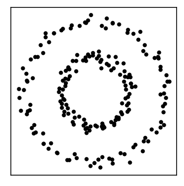
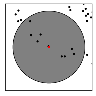
We expect to find two clusters (an inner and an outer ring) in this data set. We will at first compute the neighbourhoods for all points with respect to a radius of \(r\). Below we show the neighbourhood for the first point in the set.

r = 0.7

def point_zoom(data, point, ax):
    ax.plot(*data.T, "k.")
    ax.plot(*data[point].T, "r.")

    neighbourhood = mpl.patches.Circle(
        data[point], r,
        edgecolor="k",
        facecolor="grey"
    )
    ax.add_patch(neighbourhood)

    limit_factor = 1.2
    ax.set_xlim(data[point][0] - r * limit_factor,
                data[point][0] + r * limit_factor)
    ax.set_ylim(data[point][1] - r * limit_factor,
                data[point][1] + r * limit_factor)
    ax.set(**{
        "xticks": (),
        "yticks": (),
        "aspect": "equal"
    })

fig, ax = plt.subplots()
point_zoom(noisy_circles, 0, ax=ax)

# Calculate neighbourhoods using a k-d tree
tree = cKDTree(noisy_circles)
neighbourhoods = [set(x) for x in tree.query_ball_point(noisy_circles, r)]
for i, s in enumerate(neighbourhoods):
    # Avoid neighbour self-counting
    s.remove(i)

def check_similarity(a, b, c):
    """Check the CNN density criterion"""
    if len(a & b) >= c:
        return True
    return False

def commonn_from_neighbourhoods(
        neighbourhoods, c, yield_iterations=False):
    """Apply CNN clustering

    neighbourhoods:
        list of sets of point indices
        (neighbours of each point)
    c:
        Density reachable points need at least this many common
        nearest neighbours
    yield_iterations:
        Report state of clustering after each label assignment
    """

    n = len(neighbourhoods)              # Number of points
    visited = [False for _ in range(n)]  # Track visited
    labels = [0 for _ in range(n)]       # Output container
    queue = deque()                      # FIFO queue
    current = 1                          # Cluster count

    for point in range(n):
        # Source node
        if visited[point]:
            continue

        visited[point] = True

        neighbours = neighbourhoods[point]
        if len(neighbours) <= c:
            continue

        labels[point] = current

        if yield_iterations:
            # Get current state of clustering
            yield (point, None, current, labels, visited)

        while True:
            for member in neighbours:
                if visited[member]:
                    continue

                neighbour_neighbours = neighbourhoods[member]
                if len(neighbour_neighbours) <= c:
                    continue

                if check_similarity(neighbours, neighbour_neighbours, c):
                    labels[member] = current
                    visited[member] = True
                    queue.append(member)

                    if yield_iterations:
                        # Get current state of clustering
                        yield (point, member, current, labels, visited)

            if not queue:
                break

            point = queue.popleft()
            neighbours = neighbourhoods[point]

        current += 1

    if not yield_iterations:
        yield labels

def plt_iteration(
        data, iteration=None, ax=None, ax_props=None, color_list=None):

    if ax is None:
        fig, ax = plt.subplots()
    else:
        fig = ax.get_figure()

    ax_props_defaults = {
        "xticks": (),
        "yticks": (),
        "aspect": "equal"
    }

    if ax_props is not None:
        ax_props_defaults.update(ax_props)

    if iteration is not None:
        point, member, current, labels, visited = iteration

        if color_list is None:
            color_list = [
                "black"] + [
                    i["color"]
                    for i in islice(mpl.rcParams["axes.prop_cycle"], current)
                ]

        for cluster in range(current + 1):
            indices = np.where(np.asarray(labels) == cluster)[0]
            ax.plot(*data[indices].T, c=color_list[cluster],
                    linestyle="", marker=".")

    else:
        ax.plot(*data.T)

    ax.set(**ax_props_defaults)

class AnimatedIterations:
    """An animated scatter plot using matplotlib.animations.FuncAnimation."""
    def __init__(self, data, iterations=None):
        self.data = data
        self.iterations = iter(iterations)
        self.highlights = deque(maxlen=5)
        self.sizes = np.ones(len(self.data)) * 10

        self.fig, self.ax = plt.subplots()
        self.animation = animation.FuncAnimation(
            self.fig, self.update, frames=200, interval=100,
            init_func=self.setup_plot, blit=True
            )

    def setup_plot(self):
        """Initial drawing of the scatter plot."""
        self.scatter = self.ax.scatter(
            *self.data.T,
            s=self.sizes,
            c=np.asarray([0 for _ in range(len(self.data))]),
            cmap=mpl.colors.LinearSegmentedColormap.from_list(
                "cluster_map",
                ["black"] + [
                    i["color"]
                    for i in islice(mpl.rcParams["axes.prop_cycle"], 2)
                    ]
                ),
            vmin=0, vmax=2
            )
        # self.ax.axis([-10, 10, -10, 10])
        # For FuncAnimation's sake, we need to return the artist we'll be using
        # Note that it expects a sequence of artists, thus the trailing comma.
        return self.scatter,

    def update(self, i):
        """Update the scatter plot."""
        point, member, current, labels, visited = next(self.iterations)
        if member is None:
            self.highlights.append(point)
        else:
            self.highlights.append(member)

        for c, p in enumerate(self.highlights, 1):
            self.sizes[p] = c * 10

        # Set sizes
        self.scatter.set_sizes(self.sizes)

        # Set colors
        self.scatter.set_array(np.asarray(labels))

        # We need to return the updated artist for FuncAnimation to draw..
        # Note that it expects a sequence of artists, thus the trailing comma.
        return self.scatter,


Animation = AnimatedIterations(
    noisy_circles,
    commonn_from_neighbourhoods(neighbourhoods, 5, yield_iterations=True)
)
# Animation.animation.save('algorithm_explained/iteration.mp4', dpi=300)
plt.close()

Debug mode

In the current version of the cnnclustering package, CommonNN clustering is in detail quite differently implemented than shown in the previous section. To get a closer look at what is going on during a clustering, we provide a fitter type that can yield the state of the assignment during a clustering procedure.

clustering = cluster.Clustering(noisy_circles, fitter="bfs_debug")
print(clustering)

Clustering(input_data=InputDataExtComponentsMemoryview, fitter=FitterExtBFSDebug(ngetter=NeighboursGetterExtBruteForce(dgetter=DistanceGetterExtMetric(metric=MetricExtEuclideanReduced), sorted=False, selfcounting=True), na=NeighboursExtVectorCPPUnorderedSet, nb=NeighboursExtVectorCPPUnorderedSet, checker=SimilarityCheckerExtSwitchContains, queue=QueueExtFIFOQueue, verbose=True, yielding=True), predictor=None)

As the fit method of the debug fitter _types.FitterExtBFSDebug is returning generator, we can not invoke it directly from the Clustering object but have to call it manually.

clustering.labels = np.zeros(clustering._input_data.n_points, dtype=int)
iterations = clustering.fitter.fit(
    clustering._input_data,
    clustering._labels,
    _types.ClusterParameters(0.7, 5)
)
iterations

<generator at 0x7f14d9f89c10>

state = next(iterations)

CommonNN clustering - FitterExtBFSDebug
================================================================================
200 points
radius_cutoff                : 0.7
similarity_cutoff            : 5
similarity_cutoff_continuous : 0.0
n_member_cutoff              : 5
current_start                : 1

New source: 0
    ... new cluster 1

state

{'reason': 'assigned_source', 'init_point': 0, 'point': None, 'member': None}

state = next(iterations)

    ... loop over 15 neighbours
        ... current neighbour 0
        ... already visited

        ... current neighbour 1
        ... successful check!

state

{'reason': 'assigned_neighbour', 'init_point': 0, 'point': 0, 'member': 1}

clustering.labels

array([1, 1, 0, 0, 0, 0, 0, 0, 0, 0, 0, 0, 0, 0, 0, 0, 0, 0, 0, 0, 0, 0,
       0, 0, 0, 0, 0, 0, 0, 0, 0, 0, 0, 0, 0, 0, 0, 0, 0, 0, 0, 0, 0, 0,
       0, 0, 0, 0, 0, 0, 0, 0, 0, 0, 0, 0, 0, 0, 0, 0, 0, 0, 0, 0, 0, 0,
       0, 0, 0, 0, 0, 0, 0, 0, 0, 0, 0, 0, 0, 0, 0, 0, 0, 0, 0, 0, 0, 0,
       0, 0, 0, 0, 0, 0, 0, 0, 0, 0, 0, 0, 0, 0, 0, 0, 0, 0, 0, 0, 0, 0,
       0, 0, 0, 0, 0, 0, 0, 0, 0, 0, 0, 0, 0, 0, 0, 0, 0, 0, 0, 0, 0, 0,
       0, 0, 0, 0, 0, 0, 0, 0, 0, 0, 0, 0, 0, 0, 0, 0, 0, 0, 0, 0, 0, 0,
       0, 0, 0, 0, 0, 0, 0, 0, 0, 0, 0, 0, 0, 0, 0, 0, 0, 0, 0, 0, 0, 0,
       0, 0, 0, 0, 0, 0, 0, 0, 0, 0, 0, 0, 0, 0, 0, 0, 0, 0, 0, 0, 0, 0,
       0, 0])