Basic usage

Go to:

• Notebook configuration

• Getting started

Notebook configuration

import sys

# Optional dependencies
import matplotlib as mpl
import matplotlib.pyplot as plt

import cnnclustering
from cnnclustering import cluster

Print Python and package version information:

# Version information
print("Python: ", *sys.version.split("\n"))

print("Packages:")
for package in [mpl, cnnclustering]:
    print(f"    {package.__name__}: {package.__version__}")

Python:  3.8.8 (default, Mar 11 2021, 08:58:19)  [GCC 8.3.0]
Packages:
    matplotlib: 3.3.4
    cnnclustering: 0.4.3

We use Matplotlib to create plots. The matplotlibrc file in the root directory of the CommonNNClustering repository is used to customize the appearance of the plots.

# Matplotlib configuration
mpl.rc_file(
    "../../matplotlibrc",
    use_default_template=False
)

# Axis property defaults for the plots
ax_props = {
    "aspect": "equal"
}

# Property defaults for plotted lines
dot_props = {
    "marker": "o",
    "markeredgecolor": "k"
}

Getting started

The cnnclustering.cluster main module provides the Clustering class. An instance of this class is used to bundle input data (e.g. data points) with cluster results (cluster label assignments) alongside the clustering method (a fitter with a set of building blocks) and convenience functions for further analysis (not only in an Molecular Dynamics context). As a guiding principle, a Clustering object is always associated with one particular data set and allows varying cluster parameters.

Info: The user is also refered to the scikit-learn-extra project for an alternative API following a parameter centered approach to clustering as sklearn_extra.cluster.CommonNNClustering.

A Clustering can be initiated by passing raw input data to it. By default, this is expected to be a nested sequence, e.g. a list of lists. It will be understood as the coordinates of a number of data points in a feature space. Similar data structures, like a two-dimensional NumPy array would be acceptable, as well. It is possible to use different kinds of input data formats instead, like for example pre-computed pairwise distances, and it is described later how to do it (refer to tutorials Clustering of scikit-learn toy data sets and Advanced usage).

# 2D Data points (list of lists, 12 points in 2 dimensions)
data_points = [   # Point index
    [0, 0],       # 0
    [1, 1],       # 1
    [1, 0],       # 2
    [0, -1],      # 3
    [0.5, -0.5],  # 4
    [2,  1.5],    # 5
    [2.5, -0.5],  # 6
    [4, 2],       # 7
    [4.5, 2.5],   # 8
    [5, -1],      # 9
    [5.5, -0.5],  # 10
    [5.5, -1.5],  # 11
    ]

clustering = cluster.Clustering(data_points)

We can get a view of the input data associated with a Clustering back like this:

clustering.input_data

array([[ 0. ,  0. ],
       [ 1. ,  1. ],
       [ 1. ,  0. ],
       [ 0. , -1. ],
       [ 0.5, -0.5],
       [ 2. ,  1.5],
       [ 2.5, -0.5],
       [ 4. ,  2. ],
       [ 4.5,  2.5],
       [ 5. , -1. ],
       [ 5.5, -0.5],
       [ 5.5, -1.5]])

Info: The raw data points that we passed here to create the Clustering object are internally wrapped into a specific input data type and are stored on the instance under the _input_data attribute. Clustering.input_data is actually a shortcut for Clustering._input_data.data.

When we cluster data points, we are essentially interested in cluster label assignments for these points. The labels will be exposed as labels attribute on the instance, which is currently None because no clustering has been done yet.

clustering.labels is None

True

To cluster the points, we will use the fit method. The clustering depends on two parameters:

• radius_cutoff: Points are considered neighbours if the distance between them is not larger than this cutoff radius \(r\).

• cnn_cutoff: Points are assigned to the same cluster if they share at least this number of \(c\) common neighbours.

For the clustering procedure, we ultimately need to compute the neighbouring points with respect to the radius_cutoff for each point in the data set. Then we can determine if two points fulfill the criterion of being part of the same cluster. How this is done, can be controlled in detail but by default the input data points are assumed to be given in euclidean space and the neighbours are computed brute force. For larger data sets, it makes sense to use a different approach.

clustering.fit(radius_cutoff=2.0, cnn_cutoff=1)

-----------------------------------------------------------------------------------------------
#points   r         c         min       max       #clusters %largest  %noise    time
12        2.000     1         None      None      2         0.583     0.167     00:00:0.000
-----------------------------------------------------------------------------------------------

A clustering attempt returns and prints a comprehensive record of the cluster parameters and the outcome. You can suppress the recording with the keyword argument record=False and the printing with v=False:

• #points: Number of data points in the data set.

• r: Radius cutoff r.

• c: Common-nearest-neighour cutoff c.

• min: Member cutoff (valid clusters need to have at least this many members).

• max: Maximum cluster count (keep only the max largest clusters and disregard smaller clusters).

• #clusters: Number of identified clusters.

• %largest: Member share on the total number of points in the largest cluster.

• %noise: Member share on the total number of points identified as noise (not part of any cluster).

The min (keyword argument member_cutoff) and max (keyword argument max_clusters) only take effect in an optional post processing step when sort_by_size=True (default). Then the clusters are sorted in order by there size, so that the first cluster (cluster 1) has the highest member count. Optionally, they are trimmed in the way that valid clusters have a minimum number of members (member_cutoff) and only the largest clusters are kept (max_clusters).

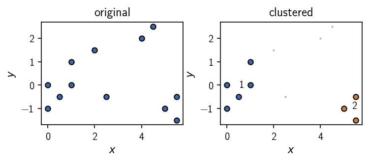
The outcome of the clustering are cluster label assignments for each point. Points classified as noise (not part of any cluster) are labeled 0. Integer labels larger than 0 indicate the membership of each point to one of the identified clusters. If clusters where sorted (sort_by_size=True), cluster 1 has the highest member count.

clustering.labels

array([1, 1, 1, 1, 1, 1, 1, 0, 0, 2, 2, 2])

The labels attribute of a cluster object always holds the result of the latest fit. All cluster results (from fits where record=True) are collected in a summary without storing the actual labels.

clustering.fit(radius_cutoff=1.5, cnn_cutoff=1, v=False)
print(*clustering.summary, sep="\n")

-----------------------------------------------------------------------------------------------
#points   r         c         min       max       #clusters %largest  %noise    time
12        2.000     1         None      None      2         0.583     0.167     00:00:0.000
-----------------------------------------------------------------------------------------------

-----------------------------------------------------------------------------------------------
#points   r         c         min       max       #clusters %largest  %noise    time
12        1.500     1         None      None      2         0.417     0.333     00:00:0.000
-----------------------------------------------------------------------------------------------

If you have Pandas installed, the summary can be transformed into a handy pandas.DataFrame.

clustering.summary.to_DataFrame()

	n_points	radius_cutoff	cnn_cutoff	member_cutoff	max_clusters	n_clusters	ratio_largest	ratio_noise	execution_time
0	12	2.0	1	<NA>	<NA>	2	0.583333	0.166667	0.000038
1	12	1.5	1	<NA>	<NA>	2	0.416667	0.333333	0.000029

A Clustering object comes with a variety of convenience methods that allow for example a quick look at a plot of data points and a cluster result.

fig, ax = plt.subplots(1, 2)

ax[0].set_title("original")
clustering.evaluate(
    ax=ax[0], original=True,
    ax_props=ax_props, plot_props=dot_props
    )

ax[1].set_title("clustered")
clustering.evaluate(
    ax=ax[1],
    ax_props=ax_props, plot_props=dot_props
    )
fig.tight_layout()