Clustering of scikit-learn toy data sets
Go to:
CommonNN clustering using …
Notebook configuration
[1]:
import sys

import matplotlib as mpl
import matplotlib.pyplot as plt
import numpy as np
import sklearn
from sklearn import datasets
from sklearn.metrics import pairwise_distances
from sklearn.neighbors import KDTree
from sklearn.preprocessing import StandardScaler

import cnnclustering
from cnnclustering import cluster, hooks
from cnnclustering import _types, _fit
[2]:
# Optional helper functionality from the benchmark module
#     https://github.com/janjoswig/CommonNNClustering-Benchmark
sys.path.insert(0, "../benchmark")
import helper_base
Print Python and package version information:
[3]:
# Version information
print("Python: ", *sys.version.split("\n"))

print("Packages:")
for package in [mpl, np, sklearn, cnnclustering]:
    print(f"    {package.__name__}: {package.__version__}")
Python:  3.8.8 (default, Mar 11 2021, 08:58:19)  [GCC 8.3.0]
Packages:
    matplotlib: 3.3.4
    numpy: 1.20.1
    sklearn: 0.24.1
    cnnclustering: 0.4.3
We use Matplotlib to create plots. The matplotlibrc file in the root directory of the CommonNNClustering repository is used to customize the appearance of the plots.
[4]:
# Matplotlib configuration
mpl.rc_file(
    "../../matplotlibrc",
    use_default_template=False
)
[5]:
# Axis property defaults for the plots
ax_props = {
    "xlabel": None,
    "ylabel": None,
    "xlim": (-2.5, 2.5),
    "ylim": (-2.5, 2.5),
    "xticks": (),
    "yticks": (),
    "aspect": "equal"
}

# Line plot property defaults
line_props = {
    "linewidth": 0,
    "marker": '.',
}
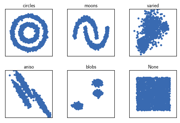
Data set generation
To see the common-nearest-neighbours (CommonNN) clustering in action, let’s have a look at a handful of basic 2D data sets from scikit-learn (like here in the scikit-learn documentation). We will cluster the data sets starting from different input data formats using the provided defaults. For more details see also the Advanced usage tutorial.
[6]:
# Data set generation parameters
np.random.seed(0)
n_samples = 2000
[7]:
# Data set generation
# Fit all datasets to the same value range
#    using `data = StandardScaler().fit_transform(data)`

# circles
noisy_circles, _ = datasets.make_circles(
    n_samples=n_samples,
    factor=.5,
    noise=.05
    )
noisy_circles = StandardScaler().fit_transform(noisy_circles)

# moons
noisy_moons, _ = datasets.make_moons(
    n_samples=n_samples,
    noise=.05
    )
noisy_moons = StandardScaler().fit_transform(noisy_moons)

# blobs
blobs, _ = datasets.make_blobs(
    n_samples=n_samples,
    random_state=8
    )
blobs = StandardScaler().fit_transform(blobs)

# None
no_structure = np.random.rand(
    n_samples, 2
    )
no_structure = StandardScaler().fit_transform(no_structure)

# aniso
random_state = 170
X, y = datasets.make_blobs(
    n_samples=n_samples,
    random_state=random_state
    )

transformation = [[0.6, -0.6], [-0.4, 0.8]]
aniso = np.dot(X, transformation)
aniso = StandardScaler().fit_transform(aniso)

# varied
varied, _ = datasets.make_blobs(
    n_samples=n_samples,
    cluster_std=[1.0, 2.5, 0.5],
    random_state=random_state
    )
varied = StandardScaler().fit_transform(varied)
[8]:
# Define cluster parameters
dsets = [ # "name", set, **parameters
    ('circles', noisy_circles, {
        'radius_cutoff': 0.5,
        'cnn_cutoff': 20,
        'member_cutoff': 100,
        'max_clusters': None
        }),
    ('moons', noisy_moons, {
        'radius_cutoff': 0.5,
        'cnn_cutoff': 20,
        'member_cutoff': 2,
        'max_clusters': None
        }),
    ('varied', varied, {
        'radius_cutoff': 0.28,
        'cnn_cutoff': 20,
        'member_cutoff': 20,
        'max_clusters': None
        }),
    ('aniso', aniso, {
        'radius_cutoff': 0.29,
        'cnn_cutoff': 30,
        'member_cutoff': 5,
        'max_clusters': None
         }),
    ('blobs', blobs, {
        'radius_cutoff': 0.4,
        'cnn_cutoff': 20,
        'member_cutoff': 2,
        'max_clusters': None
        }),
    ('None', no_structure, {
        'radius_cutoff': 0.5,
        'cnn_cutoff': 20,
        'member_cutoff': 1,
        'max_clusters': None
        }),
    ]
[9]:
# Plot the original data sets
fig, ax = plt.subplots(2, 3)
Ax = ax.flatten()

for count, (name, data, *_) in enumerate(dsets):
    Ax[count].plot(data[:, 0], data[:, 1], **line_props)
    Ax[count].set(**ax_props)
    Ax[count].set_title(f'{name}', fontsize=10, pad=4)

fig.subplots_adjust(
    left=0, right=1, bottom=0, top=1, wspace=0.1, hspace=0.3
    )
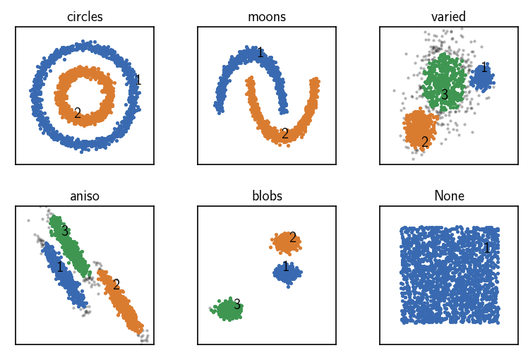
CommonNN clustering using data point coordiantes as input
[10]:
fig, ax = plt.subplots(2, 3)
Ax = ax.flatten()

for count, (name, data, params) in enumerate(dsets):

    # Default clustering initialisation
    clustering = cluster.Clustering(data)

    # Calculate neighbours brute force
    clustering.fit(**params)
    print()

    clustering.evaluate(ax=Ax[count], annotate_pos="random")
    Ax[count].set(**ax_props)
    Ax[count].set_title(f'{name}', fontsize=10, pad=4)

fig.subplots_adjust(
    left=0, right=1, bottom=0, top=1, wspace=0.1, hspace=0.3
    )
-----------------------------------------------------------------------------------------------
#points   r         c         min       max       #clusters %largest  %noise    time
2000      0.500     20        100       None      2         0.500     0.000     00:00:0.162
-----------------------------------------------------------------------------------------------


-----------------------------------------------------------------------------------------------
#points   r         c         min       max       #clusters %largest  %noise    time
2000      0.500     20        2         None      2         0.500     0.000     00:00:0.155
-----------------------------------------------------------------------------------------------


-----------------------------------------------------------------------------------------------
#points   r         c         min       max       #clusters %largest  %noise    time
2000      0.280     20        20        None      3         0.338     0.114     00:00:0.205
-----------------------------------------------------------------------------------------------


-----------------------------------------------------------------------------------------------
#points   r         c         min       max       #clusters %largest  %noise    time
2000      0.290     30        5         None      3         0.319     0.050     00:00:0.159
-----------------------------------------------------------------------------------------------


-----------------------------------------------------------------------------------------------
#points   r         c         min       max       #clusters %largest  %noise    time
2000      0.400     20        2         None      3         0.334     0.001     00:00:0.269
-----------------------------------------------------------------------------------------------


-----------------------------------------------------------------------------------------------
#points   r         c         min       max       #clusters %largest  %noise    time
2000      0.500     20        1         None      1         1.000     0.000     00:00:0.135
-----------------------------------------------------------------------------------------------

When raw input data is presented to a Clustering on creation without specifying anything else, the obtained Clustering object aggregates the needed clustering components, assuming that it got point coordinates as a sequence of sequences. The neighbourhood of a specific point will be collected brute-force by computing the (Euclidean) distances to all other points and comparing them to the radius cutoff. This will be the slowest possible approach but it has fairly conservative memory
usage.
[11]:
# Clustering components used by default ("coordinates" recipe)
print(helper_base.indent_at_parens(str(clustering)))
Clustering(
    input_data=InputDataExtComponentsMemoryview,
    fitter=FitterExtBFS(
        ngetter=NeighboursGetterExtBruteForce(
            dgetter=DistanceGetterExtMetric(
                metric=MetricExtEuclideanReduced
                ),
            sorted=False,
            selfcounting=True
            ),
        na=NeighboursExtVectorCPPUnorderedSet,
        nb=NeighboursExtVectorCPPUnorderedSet,
        checker=SimilarityCheckerExtSwitchContains,
        queue=QueueExtFIFOQueue
        ),
    predictor=None
    )
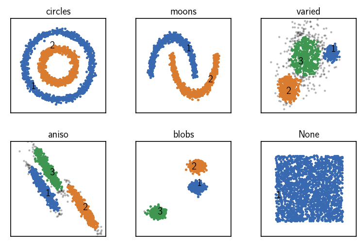
CommonNN clustering with pre-computed distances
[12]:
fig, ax = plt.subplots(2, 3)
Ax = ax.flatten()

for count, (name, data, params) in enumerate(dsets):

    # Default clustering initialisation
    clustering = cluster.Clustering(data)

    # Pre-compute distances and choose the corresponding recipe
    distances = pairwise_distances(data)
    clustering_dist = cluster.Clustering(
        distances,
        registered_recipe_key="distances"
        )

    # Use pre-computed distances
    clustering_dist.fit(**params)
    clustering._labels = clustering_dist._labels
    print()

    clustering.evaluate(ax=Ax[count], annotate_pos="random")
    Ax[count].set(**ax_props)
    Ax[count].set_title(f'{name}', fontsize=10, pad=4)

fig.subplots_adjust(
    left=0, right=1, bottom=0, top=1, wspace=0.1, hspace=0.3
    )
-----------------------------------------------------------------------------------------------
#points   r         c         min       max       #clusters %largest  %noise    time
2000      0.500     20        100       None      2         0.500     0.000     00:00:0.077
-----------------------------------------------------------------------------------------------


-----------------------------------------------------------------------------------------------
#points   r         c         min       max       #clusters %largest  %noise    time
2000      0.500     20        2         None      2         0.500     0.000     00:00:0.093
-----------------------------------------------------------------------------------------------


-----------------------------------------------------------------------------------------------
#points   r         c         min       max       #clusters %largest  %noise    time
2000      0.280     20        20        None      3         0.338     0.114     00:00:0.118
-----------------------------------------------------------------------------------------------


-----------------------------------------------------------------------------------------------
#points   r         c         min       max       #clusters %largest  %noise    time
2000      0.290     30        5         None      3         0.319     0.050     00:00:0.087
-----------------------------------------------------------------------------------------------


-----------------------------------------------------------------------------------------------
#points   r         c         min       max       #clusters %largest  %noise    time
2000      0.400     20        2         None      3         0.334     0.001     00:00:0.201
-----------------------------------------------------------------------------------------------


-----------------------------------------------------------------------------------------------
#points   r         c         min       max       #clusters %largest  %noise    time
2000      0.500     20        1         None      1         1.000     0.000     00:00:0.074
-----------------------------------------------------------------------------------------------
When raw input data is presented to a Clustering on creation in terms of a dense distance matrix, the “distances” recipe can be chosen to make the obtained Clustering object aggregate the needed clustering components. The neighbourhood of a specific point will be collected brute-force by looking up distances from the input data. This will be somewhat faster as no distances need to be calculated during the clustering but it has a high memory demand. It also allows to leverage smart
external methods for the task of the distance calculation.
[13]:
# Clustering components used by the "distance" recipe
print(helper_base.indent_at_parens(str(clustering_dist)))
Clustering(
    input_data=InputDataExtComponentsMemoryview,
    fitter=FitterExtBFS(
        ngetter=NeighboursGetterExtBruteForce(
            dgetter=DistanceGetterExtMetric(
                metric=MetricExtPrecomputed
                ),
            sorted=False,
            selfcounting=True
            ),
        na=NeighboursExtVectorCPPUnorderedSet,
        nb=NeighboursExtVectorCPPUnorderedSet,
        checker=SimilarityCheckerExtSwitchContains,
        queue=QueueExtFIFOQueue
        ),
    predictor=None
    )
CommonNN clustering with pre-computed neighbourhoods
[14]:
fig, ax = plt.subplots(2, 3)
Ax = ax.flatten()

for count, (name, data, params) in enumerate(dsets):

    clustering = cluster.Clustering(data)

    # Pre-compute neighbourhoods and choose the corresponding recipe
    tree = KDTree(data)
    neighbourhoods = tree.query_radius(
        data, r=params["radius_cutoff"], return_distance=False
        )

    clustering_neighbourhoods = cluster.Clustering(
        neighbourhoods,
        preparation_hook=hooks.prepare_neighbourhoods,
        registered_recipe_key="neighbourhoods"
        )

    # Use pre-computed neighbourhoods
    clustering_neighbourhoods.fit(**params)
    clustering._labels = clustering_neighbourhoods._labels
    print()

    clustering.evaluate(ax=Ax[count], annotate_pos="random")
    Ax[count].set(**ax_props)
    Ax[count].set_title(f'{name}', fontsize=10, pad=4)

fig.subplots_adjust(
    left=0, right=1, bottom=0, top=1, wspace=0.1, hspace=0.3
    )
-----------------------------------------------------------------------------------------------
#points   r         c         min       max       #clusters %largest  %noise    time
2000      0.500     20        100       None      2         0.500     0.000     00:00:0.036
-----------------------------------------------------------------------------------------------


-----------------------------------------------------------------------------------------------
#points   r         c         min       max       #clusters %largest  %noise    time
2000      0.500     20        2         None      2         0.500     0.000     00:00:0.052
-----------------------------------------------------------------------------------------------


-----------------------------------------------------------------------------------------------
#points   r         c         min       max       #clusters %largest  %noise    time
2000      0.280     20        20        None      3         0.338     0.114     00:00:0.064
-----------------------------------------------------------------------------------------------


-----------------------------------------------------------------------------------------------
#points   r         c         min       max       #clusters %largest  %noise    time
2000      0.290     30        5         None      3         0.319     0.050     00:00:0.039
-----------------------------------------------------------------------------------------------


-----------------------------------------------------------------------------------------------
#points   r         c         min       max       #clusters %largest  %noise    time
2000      0.400     20        2         None      3         0.334     0.001     00:00:0.149
-----------------------------------------------------------------------------------------------


-----------------------------------------------------------------------------------------------
#points   r         c         min       max       #clusters %largest  %noise    time
2000      0.500     20        1         None      1         1.000     0.000     00:00:0.032
-----------------------------------------------------------------------------------------------
When raw input data is presented to a Clustering on creation in terms of pre-computed neighbourhoods, the “neighbourhoods” recipe can be chosen to make the obtained Clustering object aggregate the needed clustering components. The neighbourhood of a specific point will looked up from the input data. This will be considerably faster and it has a lower memory demand compared to the “distances” case. It also allows to leverage smart external methods for the task of the neighbourhood
calculation.
Note, that the “neighbourhoods” recipe requires the raw neighbourhoods in the concrete format of a matrix in which the neighbourhoods of individual points are padded to the length of the largest neighbourhood. If neighbourhoods are presented in terms of a sequence of sequences (with varying length) as one would get from a tree query to sklearn.neighbors.KDTree, this can be transformed into the suitable format using the preparation hook hooks.prepare_neighbourhoods.
[15]:
# Clustering components used by the "distance" recipe
print(helper_base.indent_at_parens(str(clustering_neighbourhoods)))
Clustering(
    input_data=InputDataExtNeighbourhoodsMemoryview,
    fitter=FitterExtBFS(
        ngetter=NeighboursGetterExtLookup(
            sorted=False,
            selfcounting=True
            ),
        na=NeighboursExtVectorCPPUnorderedSet,
        nb=NeighboursExtVectorCPPUnorderedSet,
        checker=SimilarityCheckerExtSwitchContains,
        queue=QueueExtFIFOQueue
        ),
    predictor=None
    )
Common-nearest-neighbours clustering with pre-computed sorted neighbourhoods
[16]:
fig, ax = plt.subplots(2, 3)
Ax = ax.flatten()

for count, (name, data, params) in enumerate(dsets):

    clustering = cluster.Clustering(data)

    # Pre-compute and sort neighbourhoods and choose the corresponding recipe
    tree = KDTree(data)
    neighbourhoods = tree.query_radius(
        data, r=params["radius_cutoff"], return_distance=False
        )

    for n in neighbourhoods:
        n.sort()

    # Custom initialisation using a clustering builder
    clustering_neighbourhoods_sorted = cluster.Clustering(
        neighbourhoods,
        preparation_hook=hooks.prepare_neighbourhoods,
        registered_recipe_key="sorted_neighbourhoods"
        )

    # Use pre-computed neighbourhoods
    clustering_neighbourhoods_sorted.fit(**params)
    clustering._labels = clustering_neighbourhoods_sorted._labels
    print()

    clustering.evaluate(ax=Ax[count], annotate_pos="random")
    Ax[count].set(**ax_props)
    Ax[count].set_title(f'{name}', fontsize=10, pad=4)

fig.subplots_adjust(
    left=0, right=1, bottom=0, top=1, wspace=0.1, hspace=0.3
    )
-----------------------------------------------------------------------------------------------
#points   r         c         min       max       #clusters %largest  %noise    time
2000      0.500     20        100       None      2         0.500     0.000     00:00:0.003
-----------------------------------------------------------------------------------------------


-----------------------------------------------------------------------------------------------
#points   r         c         min       max       #clusters %largest  %noise    time
2000      0.500     20        2         None      2         0.500     0.000     00:00:0.004
-----------------------------------------------------------------------------------------------


-----------------------------------------------------------------------------------------------
#points   r         c         min       max       #clusters %largest  %noise    time
2000      0.280     20        20        None      3         0.338     0.114     00:00:0.006
-----------------------------------------------------------------------------------------------


-----------------------------------------------------------------------------------------------
#points   r         c         min       max       #clusters %largest  %noise    time
2000      0.290     30        5         None      3         0.319     0.050     00:00:0.004
-----------------------------------------------------------------------------------------------


-----------------------------------------------------------------------------------------------
#points   r         c         min       max       #clusters %largest  %noise    time
2000      0.400     20        2         None      3         0.334     0.001     00:00:0.011
-----------------------------------------------------------------------------------------------


-----------------------------------------------------------------------------------------------
#points   r         c         min       max       #clusters %largest  %noise    time
2000      0.500     20        1         None      1         1.000     0.000     00:00:0.004
-----------------------------------------------------------------------------------------------

Pre-computed neighbourhood information can be additionally sorted. While this has the same memory demand as using unsorted neighbourhoods, it offers the fastest clustering.
[17]:
# Clustering components used by the "distance" recipe
print(helper_base.indent_at_parens(str(clustering_neighbourhoods_sorted)))
Clustering(
    input_data=InputDataExtNeighbourhoodsMemoryview,
    fitter=FitterExtBFS(
        ngetter=NeighboursGetterExtLookup(
            sorted=True,
            selfcounting=True
            ),
        na=NeighboursExtVector,
        nb=NeighboursExtVector,
        checker=SimilarityCheckerExtScreensorted,
        queue=QueueExtFIFOQueue
        ),
    predictor=None
    )