Hierarchical clustering basics

Go to:

• Notebook configuration

• Dissimilar blobs showcase

Notebook configuration

import sys

import matplotlib as mpl
import matplotlib.pyplot as plt
import numpy as np
import pandas as pd
import sklearn
from sklearn import datasets
from sklearn.metrics import pairwise_distances
from sklearn.preprocessing import StandardScaler
from tqdm.notebook import tqdm

import cnnclustering
from cnnclustering import cluster, plot
from cnnclustering import _fit

Print Python and package version information:

# Version information
print("Python: ", *sys.version.split("\n"))

print("Packages:")
for package in [mpl, np, pd, sklearn, cnnclustering]:
    print(f"    {package.__name__}: {package.__version__}")

Python:  3.8.8 (default, Mar 11 2021, 08:58:19)  [GCC 8.3.0]
Packages:
    matplotlib: 3.3.4
    numpy: 1.20.1
    pandas: 1.2.3
    sklearn: 0.24.1
    cnnclustering: 0.4.3

We use Matplotlib to create plots. The matplotlibrc file in the root directory of the CommonNNClustering repository is used to customize the appearance of the plots.

# Matplotlib configuration
mpl.rc_file(
    "../../matplotlibrc",
    use_default_template=False
)

# Axis property defaults for the plots
ax_props = {
    "xlabel": None,
    "ylabel": None,
    "xlim": (-2.5, 2.5),
    "ylim": (-2.5, 2.5),
    "xticks": (),
    "yticks": (),
    "aspect": "equal"
}

# Line plot property defaults
line_props = {
    "linewidth": 0,
    "marker": '.',
}

# Pandas DataFrame print options
pd.set_option('display.max_rows', 1000)

Dissimilar blobs showcase

Learn in this tutorial how to use the cnnclustering.cluster module for step-wise hierarchical clusterings, where one cluster step does not deliver a satisfactory result. We will also show how to use a data set of reduced size for cluster exploration and how we can transfer the result to the original full size data set.

We will generate a sample data set of three clusters that have very different point densities and are spatially not very well separated. As we will see, it can be non-trivial (if not impossible) to extract all three clusters with a single set of cluster parameters. We will solve the problem by extracting the clusters in a two step procedure.

# Generate blobs with quite different point densities
dblobs, _ = datasets.make_blobs(
    n_samples=int(1e5),
    cluster_std=[3.5, 0.32, 1.8],
    random_state=1
    )

dblobs = StandardScaler().fit_transform(dblobs)

# Initialise clustering
clustering = cluster.Clustering(dblobs)

# Get basic information about the clustering instance
print(clustering.info())

alias: 'root'
hierarchy_level: 0
access: coordinates
points: 100000
children: None

# Plot the original data
fig, ax = plt.subplots(1, 2)
_ = clustering.evaluate(ax=ax[0], ax_props=ax_props)
plotted = clustering.evaluate(
    ax=ax[1], ax_props=ax_props,
    plot_style="contourf",
    plot_props={"levels": range(8)}
)

rect = ax[1].get_position().bounds
cax = fig.add_axes([rect[0] + rect[2] + 0.02, rect[1], 0.025, rect[3]])
cbar = fig.colorbar(plotted[-1][0], ax=ax, cax=cax, ticks=(0, 7))
cbar.set_label("density", labelpad=-15)
cbar.ax.set_yticklabels(("high", "low"))
for i in range(2):
    ax[i].set(**{"xlabel": "$x$", "ylabel": "$y$"})

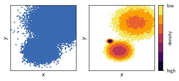
Looking at these 2D plots of the generated points above, we can already tell that this is probably not the easiest of all clustering problems. One of the three clusters is hardly visible when the data points are drawn directly (left plot). More importantly, the point density between the two narrower clusters is as high as the density within the broader cluster (right plot).

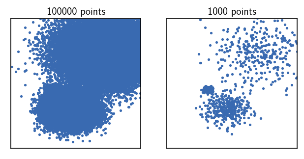
We also have generated a fairly large amount of data points. Although we can attempt to cluster the 100,000 points directly, this can be rather slow and memory intensive. For quick data exploration, it might be a good idea to perform the clustering on a reduced data set. We can predict the clustering later for the full sized set on the basis of the reduced result.

reduced_dblobs = dblobs[::100]
rclustering = cluster.Clustering(reduced_dblobs)

Here, we created a cluster object holding a smaller data set by using a point stride of 100, leaving us with only 1000 points that can be clustered very fast. By visual inspection, we can now clearly spot three point clouds.

# Plot the reduced data
fig, Ax = plt.subplots(1, 2)
_ = clustering.evaluate(ax=Ax[0], ax_props=ax_props)
_ = rclustering.evaluate(ax=Ax[1], ax_props=ax_props)
Ax[0].set_title(f"{clustering._input_data.n_points} points", fontsize=10, pad=4)
Ax[1].set_title(f"{rclustering._input_data.n_points} points", fontsize=10, pad=4)

Text(0.5, 1.0, '1000 points')

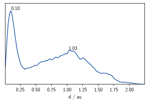
When we pre-calculate pairwise point distances, we can plot the distribution of distances. This can give us a very basic estimate for a reasonable radius cutoff as one of the cluster parameters. For globular clusters, each cluster should be visible as a peak in the distance distribution around a value that is very roughly equivalent to the radius of the point cloud. We also expect a peak for each pair of clusters, roughly corresponding to the distance between the cluster centers. For more complicated data sets this approximation is not valid, but we can still get a feeling for the value range of meaningful radius cutoffs.

In general, we want to pick a rather small radius that allows us to estimate point density with a comparably high resolution. If we pick a too small radius, however, the clustering can become sensitive to (random) fluctuations in the point density which yields probably meaningless clusters.

distances = pairwise_distances(rclustering.input_data)
distance_rclustering = cluster.Clustering(distances, registered_recipe_key="distances")

fig, ax = plt.subplots()
_ = plot.plot_histogram(ax, distances.flatten(), maxima=True, maxima_props={"order": 5})

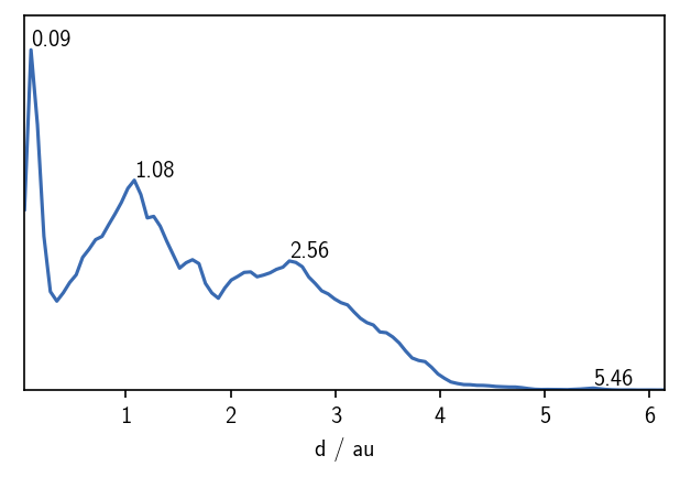
As a handy rational for a first guess on a suitable radius cutoff, we can use the first maximum in the just plotted distance distribution. For larger numbers of points, the radius can be usually smaller than for poorly sampled data sets. In this particular example, we could start with a radius cutoff of \(r\approx 0.3\) considering that we have a low number of points in the reduced data set. With this radius fixed, we can than vary the common-nearest-neighbours cutoff \(c\) to tune the density threshold for the clustering.

Parameter scan

Blindly starting to cluster a data set in a happy-go-lucky attempt may already lead to a satisfactory result in some cases, but let’s tackle this problem in a more systematic way to see how different cluster parameters effect the outcome. A scan of a few parameters shows that it is difficult to extract the three clusters at once with one parameter set. We also apply a member cutoff of 10 to prevent that we obtain clusters that are definitely too small.

r = 0.3

for c in tqdm(range(101)):
    # fit from pre-calculated distances
    distance_rclustering.fit(r, c, member_cutoff=10, v=False)

Each cluster result will be added to the summary attribute of our cluster object.

print(*distance_rclustering.summary[:5], sep="\n")

-----------------------------------------------------------------------------------------------
#points   r         c         min       max       #clusters %largest  %noise    time
1000      0.300     0         10        None      1         0.979     0.021     00:00:0.028
-----------------------------------------------------------------------------------------------

-----------------------------------------------------------------------------------------------
#points   r         c         min       max       #clusters %largest  %noise    time
1000      0.300     1         10        None      1         0.965     0.035     00:00:0.026
-----------------------------------------------------------------------------------------------

-----------------------------------------------------------------------------------------------
#points   r         c         min       max       #clusters %largest  %noise    time
1000      0.300     2         10        None      1         0.950     0.050     00:00:0.026
-----------------------------------------------------------------------------------------------

-----------------------------------------------------------------------------------------------
#points   r         c         min       max       #clusters %largest  %noise    time
1000      0.300     3         10        None      2         0.667     0.065     00:00:0.027
-----------------------------------------------------------------------------------------------

-----------------------------------------------------------------------------------------------
#points   r         c         min       max       #clusters %largest  %noise    time
1000      0.300     4         10        None      3         0.665     0.087     00:00:0.027
-----------------------------------------------------------------------------------------------

If you have pandas installed, you can convert the summary to a nice table as a pandas.DataFrame. This makes the analysis of the cluster results more convenient. We can for example specifically look for clusterings with three obtained clusters and where the largest cluster does not hold much more than a third of the points.

# Get summary sorted by number of identified clusters
df = distance_rclustering.summary.to_DataFrame().sort_values('n_clusters')

# Show cluster results where we have 3 clusters
df[(df.n_clusters == 3)].sort_values(["radius_cutoff", "cnn_cutoff"])

	n_points	radius_cutoff	cnn_cutoff	member_cutoff	max_clusters	n_clusters	ratio_largest	ratio_noise	execution_time
4	1000	0.3	4	10	<NA>	3	0.665	0.087	0.026910
7	1000	0.3	7	10	<NA>	3	0.656	0.150	0.027577
8	1000	0.3	8	10	<NA>	3	0.652	0.182	0.027540
9	1000	0.3	9	10	<NA>	3	0.650	0.198	0.028366
10	1000	0.3	10	10	<NA>	3	0.645	0.210	0.027894
18	1000	0.3	18	10	<NA>	3	0.620	0.298	0.030822
20	1000	0.3	20	10	<NA>	3	0.614	0.326	0.031672
21	1000	0.3	21	10	<NA>	3	0.609	0.336	0.032149
22	1000	0.3	22	10	<NA>	3	0.602	0.360	0.032596
25	1000	0.3	25	10	<NA>	3	0.341	0.399	0.031528

The summary shows indeed that we got clustering with 3 clusters (as desired) for some parameter combinations. Apart from the number of clusters, it is, however often also of interest, how many data points ended up in the clusters and how many are considered outliers (noise). In this case we expect 3 clusters of more or less equal size (member wise) and we may be interested in keeping the outliers-level low. In the results giving 3 clusters, in one case the largest cluster entails one third of the data points (which is good), but the noise level is around 40 % (which is most likely not what we want). Let’s plot a few results to see what is going on here.

# Cluster attempts in comparison
fig, ax = plt.subplots(2, 2)
Ax = ax.flatten()
for i, pair in enumerate([(0.3, 4), (0.3, 10), (0.3, 20), (0.3, 25)]):
    distance_rclustering.fit(*pair, member_cutoff=10, record=False, v=False)
    rclustering._labels = distance_rclustering._labels

    _ = rclustering.evaluate(ax=Ax[i], ax_props=ax_props)
    Ax[i].set_title(f'{pair[0]}, {pair[1]}', fontsize=10, pad=4)

fig.subplots_adjust(
    left=0.2, right=0.8, bottom=0, top=1, wspace=0, hspace=0.3
    )

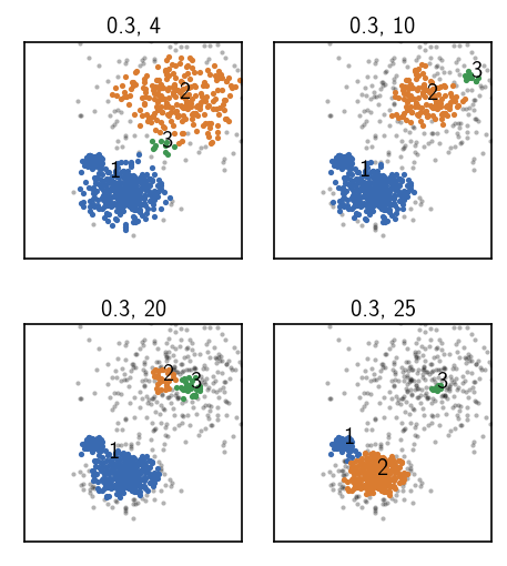
None of the above attempts was able to achieve a split into 3 clusters as we wanted it. One could now try to tinker around with the parameters a bit more (which is probably not very fruitful), or resort to hierarchical clustering. As we see in the plots above (lower right and upper right), two different parameter pairs are leading to splits in different regions of the data, separating either the lowest density cluster from the rest or separating the two denser clusters. So why not apply both of them, one after the other.

Before we do this let’s have another close look at the cluster results we obtained. Using the summarize method of a cluster object, we can visualize a summary table in a 2D contour plot, to evaluate a few quality measures versus the input parameters radius cutoff (r) and similarity criterion (c):

• number of identified clusters

• members in the largest cluster

• points classified as outliers

• computational time of the fit

Let’s also throw in a few more different values for the radius cutoff into the mix.

for r in tqdm([x/10 for x in range(1, 11) if x != 3]):
    for c in range(101):
        # fit from pre-calculated distances
        distance_rclustering.fit(r, c, member_cutoff=10, v=False)

# Computing time
fig, ax = plt.subplots()
contour = distance_rclustering.summarize(
    ax=ax, quantity="execution_time",
    contour_props={
        "levels": 50,
        }
    )[2][0]
colorbar = fig.colorbar(mappable=contour, ax=ax)
colorbar.set_label("time / s")

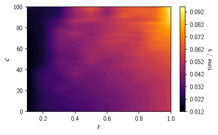
From the time vs. r/c plot we can see how the total clustering time depends in particular on the neighbour search radius. Larger radii result in larger neighbour lists for each point, increasing the processing time, so if one has the choice, smaller values for r should be preferred.

# Noise level
fig, ax = plt.subplots()
contour = distance_rclustering.summarize(
    ax=ax, quantity="ratio_noise",
    contour_props={
        "levels": [x/100 for x in range(101)],
        }
)[2][0]
colorbar = fig.colorbar(mappable=contour, ax=ax, ticks=(0, 0.5, 1))
colorbar.set_label("noise / %")

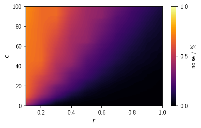
The ratio of outlier-points depends on the search radius r as well as on the similarity criterion c and increases continuously with the set density threshold. For high density thresholds (low r and high c) the noise ratio is comparably large. The desired amount of noise depends much on the nature of the underlying data set.

# Largest cluster
fig, ax = plt.subplots()
contour = distance_rclustering.summarize(
    ax=ax, quantity="ratio_largest",
    contour_props={
        "levels": [x/100 for x in range(101)],
        }
)[2][0]
colorbar = fig.colorbar(mappable=contour, ax=ax, ticks=(0, 0.5, 1))
colorbar.set_label("largest / %")

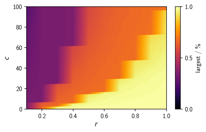
The ratio of points assigned to the largest cluster shows a similar trend as the noise-ratio, only that it changes in a rather step-wise manner. This view could give a good hint towards reasonable parameter combinations if one already has an idea about the expected cluster size. It also shows for which parameters we do not observe any splitting (about 100 % of the points are in the largest cluster).

# Number of clusters
show_n = 5

fig, ax = plt.subplots()
contour = distance_rclustering.summarize(
    ax=ax, quantity="n_clusters",
    contour_props={
        "levels": np.arange(-0.5, show_n + 1.5, 1),
        "vmin": 0,
        "vmax": show_n,
        "extend": "max"
    }
)[2][0]
colorbar = fig.colorbar(mappable=contour, ax=ax, ticks=range(0, show_n + 1, 1))
colorbar.set_label("# clusters")

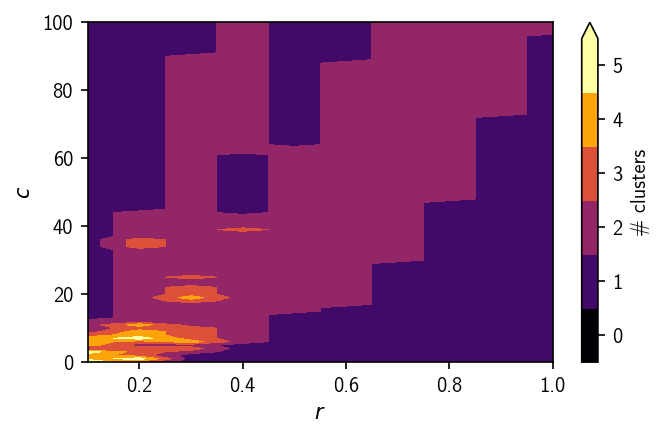
The probably most telling view is given by the number of clusters plots. The analysis demonstrates nicely that for this data set a splitting into 3 meaningful clusters is hard to achieve. With increased density threshold, the number of obtained clusters does at first increase before it drops again when low density clusters become part of the noise. In general, clusterings that are stable over a wider range of parameter combinations tend to be more meaningful.

Hierarchical clustering

To use the hierarchical approach on clustering this data set, we will apply a pair of cluster parameters that will extract the lesser dense region of the data as an isolated cluster in a first step. That means we choose a comparably low value for the similarity criterion c. We can refer to these parameters as soft parameters, leaving the more dense regions of the data untouched and in one cluster. Remember that density in terms of common-nearest-neighbour clustering is estimated as the number of common neighbours within the neighbourhood intersection of two points with respect to a radius r. More common neighbours (higher similarity cutoff c) and/or a smaller neighbourhood radius (smaller r) will result in a higher density requirement. To make this more clear let’s have a look again at some clusterings.

# Cluster attempts in comparison
fig, ax = plt.subplots(2, 2)
Ax = ax.flatten()
for i, pair in enumerate([(0.3, 1), (0.3, 3), (0.3, 40), (0.3, 100)]):
    distance_rclustering.fit(*pair, member_cutoff=10, record=False, v=False)
    rclustering._labels = distance_rclustering._labels
    _ = rclustering.evaluate(ax=Ax[i], ax_props=ax_props)
    Ax[i].set_title(f'{pair[0]}, {pair[1]}', fontsize=10, pad=4)

fig.subplots_adjust(
    left=0.2, right=0.8, bottom=0, top=1, wspace=0, hspace=0.3
    )

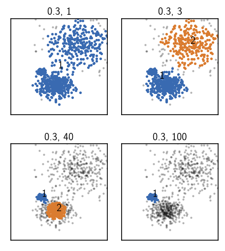
For these clustering, we again keep the radius fixed while we increase the similarity cutoff and therefore the density threshold.

Upper left: Choosing a low (soft) threshold, results in no cluster splitting. The data set as a whole forms clusters in which the point density is at least as high as our density requirement.

Upper right: When we increase the density requirement just a bit, we observe a splitting between the broadly distributed lower density cluster and the more dense clusters. Within both the resulting clusters the point density is higher than required by the parameters but they are separated by a low density region and therefore split. This parameter set can be used for the first step of the hierarchical clustering.

Lower left: Increasing the density requirement further, eventually leads to a splitting between the two denser clusters. At his point, the broader low density cluster has already vanished into noise because the density within this cluster is lower than the density between the just split denser clusters. We could use this parameter set in a second hierarchical clustering step.

lower right: Choosing even harder parameters leaves only the densest cluster. The second densest cluster falls into the noise region.

The central element of the hierarchical cluster functionality is the isolate method of a Clustering object. After a clustering (with soft parameters) we can freeze the result before we start to re-cluster.

# After the first step, we need to isolate the cluster result
rclustering.fit(0.3, 3, member_cutoff=10, record=False, v=False)
rclustering.isolate()

The isolate method will create a new Clustering object (a child clustering) for every cluster of a cluster result. In our case we get two new child clusters (plus one for outliers). The clusters are stored in a dictionary under the children attribute of the parent Clustering object. The children dictionary of the data after isolation holds a Clustering object for each cluster found in the last step.

{k: type(v) for k, v in rclustering.children.items()}

{1: cnnclustering.cluster.Clustering,
 2: cnnclustering.cluster.Clustering,
 0: cnnclustering.cluster.Clustering}

Since we will use different cluster parameters now for different clusters it would be nice to have something to keep the overview of which cluster has been identified under which parameters. This information is provided by the meta attribute on the object that stores the cluster label assignments on the Clustering which we get with Clustering._labels. Note that this is different to Clustering._labels which only return the actual labels in form of a NumPy array. The label meta information tells us three things:

• origin: How have these labels been assigned? The entry "fit" means, they were obtained by a regular clustering.

• reference: This is a related clustering object, i.e. the object that is associated to the data for which the labels are valid. For "fitted" labels this is a reference to the clustering object itself that carries the labels.

• params: This is a dictionary stating the cluster parameters (r, c) that led to each cluster. For "fitted" labels, each cluster has the same parameters.

print(*(f"{k}: {v!r}" for k, v in rclustering._labels.meta.items()), sep="\n")

params: {1: (0.3, 3), 2: (0.3, 3)}
reference: <weakproxy at 0x7f88c0c44720 to Clustering at 0x7f88c61d2ac0>
origin: 'fit'

Every single isolated child cluster is represented by a full-fledged, completely functional Clustering object itself. When we want to re-cluster a child Clustering, this is no different to clustering a parent Clustering.

child1 = rclustering.children[1]
print(child1.info())  # Child cluster 1

alias: 'rootroot - 1'
hierarchy_level: 1
access: coordinates
points: 667
children: None

Note, that the hierarchy_level in the above overview has increased to 1. We can again plot the distance distribution within this child cluster to see how this changed.

distances_child1 = pairwise_distances(child1.input_data)
fig, ax = plt.subplots()
_ = plot.plot_histogram(ax, distances_child1, maxima=True, maxima_props={"order": 5})

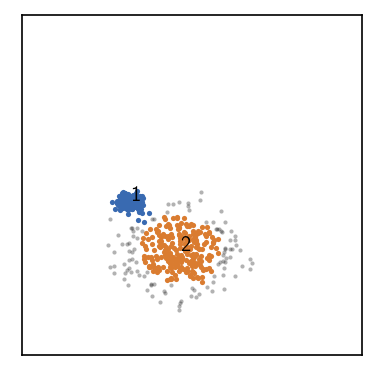
And then we can attempt the second clustering step.

# Now cluster the child cluster
fig, ax = plt.subplots()
child1.fit(0.3, 30, member_cutoff=10)
_ = child1.evaluate(ax=ax, ax_props=ax_props)

-----------------------------------------------------------------------------------------------
#points   r         c         min       max       #clusters %largest  %noise    time
667       0.300     30        10        None      2         0.505     0.153     00:00:0.036
-----------------------------------------------------------------------------------------------

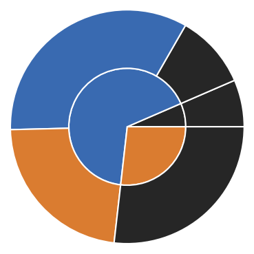
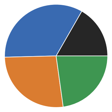
As a little extra feature a Clustering object has a pie method that allows to visualize the current state and splitting on the different hierarchy levels as a pie-diagram (from level 0 in the middle to lower levels to the outside).

# The cluster hierarchy can be visualised as pie diagram
fig, ax, *plotted = rclustering.pie(
    pie_props={
        "radius": 0.15,
        "wedgeprops": dict(width=0.15, edgecolor='w')
    }
)
ax.set_xlim(-0.3, 0.3)
ax.set_ylim(-0.3, 0.3)

(-0.3, 0.3)

Alternatively, a hierarchical tree can be drawn using the tree method.

# Tree shows only isolated clusterings
child1.isolate()
rclustering.tree()

(<Figure size 750x450 with 1 Axes>, <AxesSubplot:>)

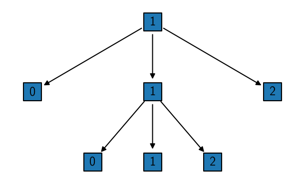
Now that we have isolated one cluster in the first step and two others in a further splitting on a lower hierarchy level, the last step that remains, is to put everything back together. This can be done automatically by calling reel on the parent cluster object into which the child cluster results should be integrated.

# Wrap up the hierarchical clustering and integrate the child clusters into
# the parent cluster
rclustering.reel()

# Manually sort clusters by size (make largest be cluster number 1)
rclustering._labels.sort_by_size()

rclustering._children = None
fig, ax, *plotted = rclustering.pie(
    pie_props={
        "radius": 0.3,
        "wedgeprops": dict(width=0.3, edgecolor='w')
    }
)
ax.set_xlim(-0.3, 0.3)
ax.set_ylim(-0.3, 0.3)

(-0.3, 0.3)

fig, ax = plt.subplots()
_ = rclustering.evaluate(ax=ax, ax_props=ax_props)

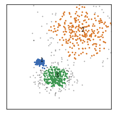
Label prediction

Now, the parameter information saved for the labels becomes useful as they differ for the clusters from different clustering steps.

rclustering._labels.meta

{'params': {2: (0.3, 3), 3: (0.3, 30), 1: (0.3, 30)},
 'reference': <cnnclustering.cluster.Clustering at 0x7f88c0c44720>,
 'origin': 'reel'}

print("Label", "r", "n", sep="\t")
print("-" * 20)
for k, v in sorted(rclustering._labels.meta["params"].items()):
    print(k, *v, sep="\t")

Label   r       n
--------------------
1       0.3     30
2       0.3     3
3       0.3     30

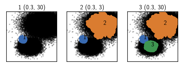
The cluster result is satisfying. But we have clustered only a reduced set of 1000 points. We would like to predict the cluster label assignment for the full 100,000 points on the basis of the reduced set assignments. This we can do with the predict method of a cluster object. We call predict with another cluster object for which labels should be predicted as an argument. Similar to a regular fit we need to compute neighbourhoods for the points that need assignment, but this time we need relative neighbourhoods between two data sets. We want to compute the neighbouring points in the small set rclustering for the points in the big set clustering. When we predict labels we should do the prediction separately for the clusters because the assignment parameters differ. This is where the label info comes in handy showing us the parameters used for the fit as an orientation.

Info: A cluster label prediction requires a Predictor in the same way as a clustering requires a Fitter. See tutorial Advanced usage for details.

rclustering._predictor = _fit.PredictorFirstmatch(
    rclustering._fitter._neighbours_getter,
    rclustering._fitter._neighbours_getter,
    rclustering._fitter._neighbours,
    rclustering._fitter._neighbour_neighbours,
    rclustering._fitter._similarity_checker,
)

fig, Ax = plt.subplots(1, 3)

r = 0.3; c = 30
rclustering.predict(clustering, r, c, clusters=[1], purge=True)
_ = clustering.evaluate(ax=Ax[0], ax_props=ax_props)
Ax[0].set_title(f'1 {(r, c)}', fontsize=10, pad=4)

r = 0.3; c = 3
rclustering.predict(clustering, r, c, clusters=[2])
_ = clustering.evaluate(ax=Ax[1], ax_props=ax_props)
Ax[1].set_title(f'2 {(r, c)}', fontsize=10, pad=4)

r = 0.3; c = 30
rclustering.predict(clustering, r, c, clusters=[3])
_ = clustering.evaluate(ax=Ax[2], ax_props=ax_props)
Ax[2].set_title(f'3 {(r, c)}', fontsize=10, pad=4)

Text(0.5, 1.0, '3 (0.3, 30)')

print("Label", "r", "n", sep="\t")
print("-" * 20)
for k, v in sorted(clustering._labels.meta["params"].items()):
    print(k, *v, sep="\t")

Label   r       n
--------------------
1       0.3     30
2       0.3     3
3       0.3     30