Molecular dynamics application example
[42]:
from pathlib import Path
import sys

import numpy as np
import matplotlib.pyplot as plt
import matplotlib as mpl
from sklearn import datasets
from sklearn.metrics import pairwise_distances
from sklearn.preprocessing import StandardScaler

from cnnclustering import cluster
from cnnclustering import plot
import csmsm
This notebook was created using Python 3.8.
[2]:
# Version information
print(sys.version)
3.8.8 (default, Mar 11 2021, 08:58:19)
[GCC 8.3.0]
Notebook configuration
[3]:
# Matplotlib configuration
mpl.rc_file(
    "../../matplotlibrc",
    use_default_template=False
)
[4]:
# Axis property defaults for the plots
ax_props = {
    "xlabel": None,
    "ylabel": None,
    "xlim": (-2.5, 2.5),
    "ylim": (-2.5, 2.5),
    "xticks": (),
    "yticks": (),
    "aspect": "equal"
}

# Line plot property defaults
line_props = {
    "linewidth": 0,
    "marker": '.',
}
Helper functions
[30]:
def draw_evaluate(clustering, axis_labels=False, plot_style="dots"):
    fig, Ax = plt.subplots(
        1, 3,
        figsize=(mpl.rcParams['figure.figsize'][0],
                 mpl.rcParams['figure.figsize'][1] * 0.5)
        )

    for dim in range(3):
        dim_ = (dim * 2, dim * 2 + 1)

        ax_props_ = {k: v for k, v in ax_props.items()}
        if axis_labels:
            ax_props_.update(
                {"xlabel": dim_[0] + 1, "ylabel": dim_[1] + 1}
            )

        _ = clustering.evaluate(
            ax=Ax[dim],
            plot_style=plot_style,
            ax_props=ax_props_,
            dim=dim_
            )

        Ax[dim].yaxis.get_label().set_rotation(0)
The C-type lection receptor langerin
Let’s read in some “real world” data for this example. We will work with a 6D projection from a classical MD trajectory of the C-type lectin receptor langerin that was generated by the dimension reduction procedure TICA.
[33]:
langerin = cluster.prepare_clustering(
    np.load("md_example/langerin_projection.npy", allow_pickle=True)
    )
After creating a Clustering instance, we can print out basic information about the data. The projection comes in 116 parts of individual independent simulations. In total we have about 26,000 data points in this set representing 26 microseconds of simulation time at a sampling timestep of 1 nanoseconds.
[36]:
print(langerin)
hierarchy_level: 0
input_data_kind: points
points: 26528
children: None
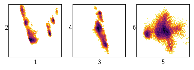
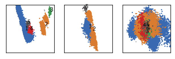
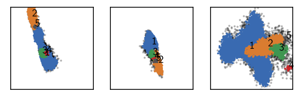
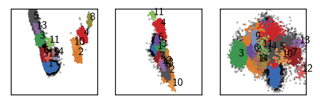
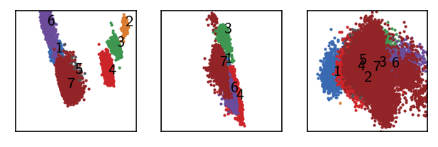
Dealing with six data dimensions we can still visualise the data quite well.
[37]:
draw_evaluate(langerin, axis_labels=True, plot_style="contourf")
A quick look on the distribution of distances in the set gives us a first feeling for what might be a suitable value for the neighbour search radius r.
[43]:
distances = pairwise_distances(langerin.input_data)

fig, ax = plt.subplots()
_ = plot.plot_histogram(ax, distances.flatten(), maxima=True, maxima_props={"order": 5})
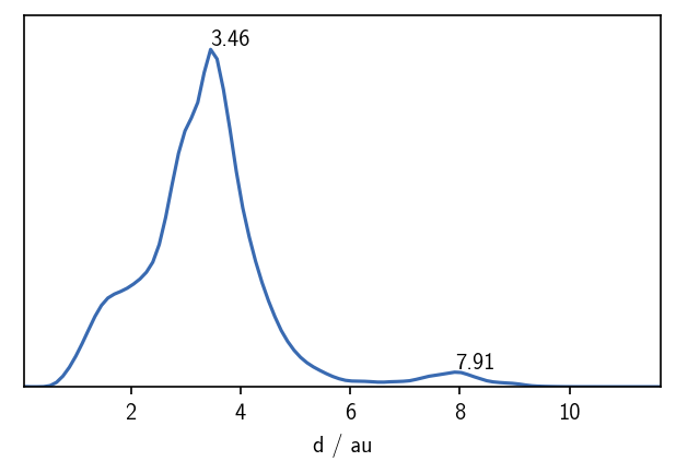
We can expect a split of the data into clusters for values of r of roughly 2 or lower. The maximum in the distribution closest to 0 defines a reasonable value range for \(r\). We can also get a feeling for what values c could take by checking the number of neighbours each point has for a given search radius.
[54]:
range_ = (-0.5, 1000.5)
bins_ = len(range(int(range_[0] + 0.5), int(range_[1] - 0.5))) + 1
fig, ax = plt.subplots(2, 1)
radii = [0.2, 0.5, 0.75, 1]
for radius in radii:
    n_neighbours = [x[(x < radius ) & (x > 0)].shape[0] for x in distances]
    H, e = np.histogram(
        n_neighbours,
        bins = bins_,
        range=range_
    )
    e = (e[:-1] + e[1:]) / 2
    ax[0].plot(e, H)
    ax[1].plot(e, H)

ax[0].set(**{
    "title": "Number of neighbours with respect to a radius",
    "xlim": (range_[0] + 0.5, (range_[1] - 0.5) / 100),
    "ylabel": "number of points                    "
    })
ax[1].set(**{
    "xlim": (1, range_[1] - 0.5),
    "xscale": "log",
    "yscale": "log",
    "xlabel": "number of neighbours"
    })

ax[0].legend(radii, fancybox=False, framealpha=1, edgecolor="k")

fig.tight_layout(pad=0.1)
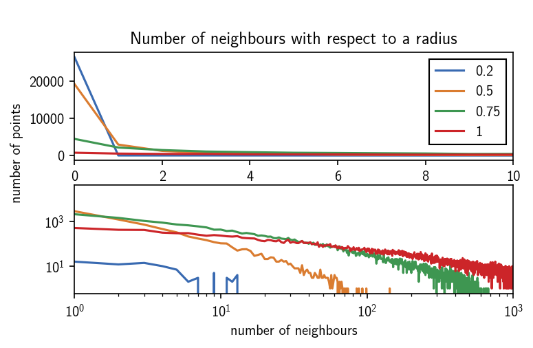
In the radius value regime of 1 and lower the number of neighbours per point quickly approaches the order of number of points in the whole data set. We can look at these plots as an upper bound for c if r gets lower. Values of c larger than 100 wont make sense for radii below 0.5. We can also see that for a radius of 0.2, a lot of the data points has no neighbour at all.
Clustering root data
[ ]:
langerin.fit()
Let’s attempt a first clustering step with a relatively low density criterion (large r cutoff, low number of common neighbours c). When we cluster, we can judge the outcome by how many clusters we obtain and how many points end up as being classified as noise. For the first clustering steps, it can be a good idea to start with a low density cutoff and then increase it gradually. As we choose higher density criteria the number of resulting clusters will rise and so will the noise level. We need to find the point where we yield a large number of (reasonably sized) clusters without loosing relevant information in the noise. Keep in mind that the ideal number of clusters and noise ratio are not definable and highly dependend on the nature of the data:
[ ]:
c = 20

for r in [2, 1, 0.8]:
    langerin.fit(r, c)
[118]:
langerin.fit(2, 5)
draw_evaluate(langerin_reduced)
Execution time for call of fit: 0 hours, 0 minutes, 50.9977 seconds
--------------------------------------------------------------------------------
#points   R         C         min       max       #clusters %largest  %noise
26528     2.000     5         2         None      3         0.983     0.000
--------------------------------------------------------------------------------
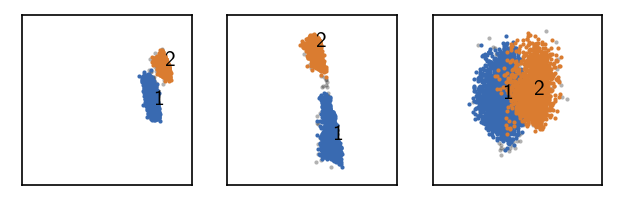
Low number of clusters and no noise points. We can push this a bit further.
[74]:
langerin_reduced.fit(1, 5, policy="progressive")
draw_evaluate(langerin_reduced)
Execution time for call of fit: 0 hours, 0 minutes, 17.9091 seconds
--------------------------------------------------------------------------------
#points   R         C         min       max       #clusters %largest  %noise
26528     1.000     5         2         None      5         0.714     0.001
--------------------------------------------------------------------------------
Two more clusters and still little noise. There is room for more. At this point we choose a member_cutoff of 10 for the fit, ensuring that we do not yield very small, meaningless clusters.
[119]:
langerin_reduced.fit(0.5, 5, policy="progressive", member_cutoff=10)
draw_evaluate(langerin_reduced)
Execution time for call of fit: 0 hours, 0 minutes, 6.1926 seconds
--------------------------------------------------------------------------------
#points   R         C         min       max       #clusters %largest  %noise
26528     0.500     5         10        None      7         0.710     0.011
--------------------------------------------------------------------------------
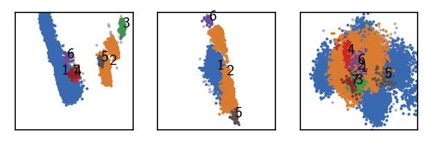
This looks good so far. There is no point in going any further at this stage. If we reduce r even more, we begin to loose clusters again into noise:
[83]:
langerin_reduced.fit(0.4, 5, policy="progressive", member_cutoff=10)
draw_evaluate(langerin_reduced)
Execution time for call of fit: 0 hours, 0 minutes, 2.9209 seconds
--------------------------------------------------------------------------------
#points   R         C         min       max       #clusters %largest  %noise
26528     0.400     5         10        None      9         0.681     0.029
--------------------------------------------------------------------------------
Clustering hierarchy level 1
We saw that parts of the data could be splitted further, but that increasing the density criterion leads to possible loss of relevant information in other data areas. Especially the first cluster can obviously be splitted further. Let’ recluster it applying a higher density criterion. For this we first need to freeze this cluster result and isolate the obtained clusters into individual child cluster objects.
[120]:
# Lets make sure we work on the correctly clustered object
print("Label", "r", "c", sep="\t")
print("-" * 20)
for k, v in sorted(langerin_reduced.labels.info.params.items()):
    print(k, *v, sep="\t")
Label   r       c
--------------------
1       0.5     5
2       0.5     5
3       0.5     5
4       0.5     5
5       0.5     5
6       0.5     5
7       0.5     5
[121]:
# Freeze this cluster result
langerin_reduced.isolate()
current = c1 = langerin_reduced.children[1]
By default, the isolation assigns an alias to each child cluster that reveals its origin. In this case “root - 1”, translates to the first child cluster of the root data.
[122]:
current
[122]:
CNN clustering object (root - 1)
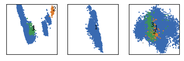
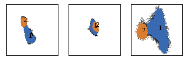
We now cluster the first child cluster from this current cluster result with increased density criteria.
[123]:
# Recluster first cluster from last step
current.data.points.cKDTree()  # We pre-compute neighbourhoods here
r = 0.4
current.calc_neighbours_from_cKDTree(r=r)
current.fit(r, 10, member_cutoff=10)
draw_evaluate(current)
Execution time for call of fit: 0 hours, 0 minutes, 0.2149 seconds
--------------------------------------------------------------------------------
#points   R         C         min       max       #clusters %largest  %noise
18839     0.400     10        10        None      3         0.946     0.029
--------------------------------------------------------------------------------
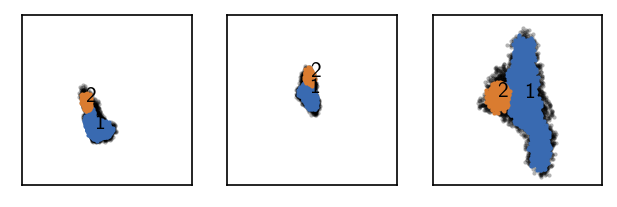
Good …
[126]:
# Recluster first cluster from last step
current.data.points.cKDTree()  # We pre-compute neighbourhoods here
r = 0.375
current.calc_neighbours_from_cKDTree(r=r)
current.fit(r, 10, member_cutoff=10)
draw_evaluate(current)
Execution time for call of fit: 0 hours, 0 minutes, 0.2091 seconds
--------------------------------------------------------------------------------
#points   R         C         min       max       #clusters %largest  %noise
18839     0.375     10        10        None      5         0.825     0.041
--------------------------------------------------------------------------------

Better …
[125]:
# Recluster first cluster from last step
current.data.points.cKDTree()  # We pre-compute neighbourhoods here
r = 0.3
current.calc_neighbours_from_cKDTree(r=r)
current.fit(r, 10, member_cutoff=10)
draw_evaluate(current)
Execution time for call of fit: 0 hours, 0 minutes, 0.1514 seconds
--------------------------------------------------------------------------------
#points   R         C         min       max       #clusters %largest  %noise
18839     0.300     10        10        None      5         0.774     0.114
--------------------------------------------------------------------------------
Probably to much! Let’s keep the second last try.
We can also work on the second cluster of the first split.
[127]:
current = c2 = langerin_reduced.children[2]
[128]:
# Recluster second cluster from last step
current.data.points.cKDTree()  # We pre-compute neighbourhoods here
r = 0.4
current.calc_neighbours_from_cKDTree(r=r)
current.fit(r, 5, member_cutoff=10)
draw_evaluate(current)
Execution time for call of fit: 0 hours, 0 minutes, 0.0485 seconds
--------------------------------------------------------------------------------
#points   R         C         min       max       #clusters %largest  %noise
6993      0.400     5         10        None      2         0.615     0.013
--------------------------------------------------------------------------------
Clustering hierarchy level 2
The re-clustered data points still may be clustered further.
[129]:
current = c1
[130]:
# Lets make sure we work on the correctly clustered object
print("Label", "r", "c", sep="\t")
print("-" * 20)
for k, v in sorted(current.labels.info.params.items()):
    print(k, *v, sep="\t")
Label   r       c
--------------------
1       0.375   10
2       0.375   10
3       0.375   10
4       0.375   10
5       0.375   10
[131]:
current
[131]:
CNN clustering object (root - 1)
[132]:
current.isolate()
current = c1_1 = current.children[1]
[133]:
current
[133]:
CNN clustering object (root - 1 - 1)
[134]:
# Recluster first cluster from last step
current.data.points.cKDTree()  # We pre-compute neighbourhoods here
r = 0.28
# current.calc_neighbours_from_cKDTree(r=r)
current.fit(r, 15, member_cutoff=10)
draw_evaluate(current)
Execution time for call of fit: 0 hours, 0 minutes, 14.5640 seconds
--------------------------------------------------------------------------------
#points   R         C         min       max       #clusters %largest  %noise
15541     0.280     15        10        None      2         0.676     0.142
--------------------------------------------------------------------------------
Clustering hierarchy level 3
And on it goes …
[135]:
current.isolate()
current = c1_1_1 = current.children[1]
[136]:
# Recluster first cluster from last step
current.data.points.cKDTree()  # We pre-compute neighbourhoods here
r = 0.22
current.calc_neighbours_from_cKDTree(r=r)
current.fit(r, 15, member_cutoff=10)
draw_evaluate(current)
Execution time for call of fit: 0 hours, 0 minutes, 0.0792 seconds
--------------------------------------------------------------------------------
#points   R         C         min       max       #clusters %largest  %noise
10506     0.220     15        10        None      2         0.650     0.309
--------------------------------------------------------------------------------
Merge hierarchy levels
We want to leave it with that for the moment. We can visualise our cluster hierarchy to get an overview.
[137]:
# Cluster hierarchy as pie diagram (hierarchy level increasing from the center outwards)
_ = langerin_reduced.pie()
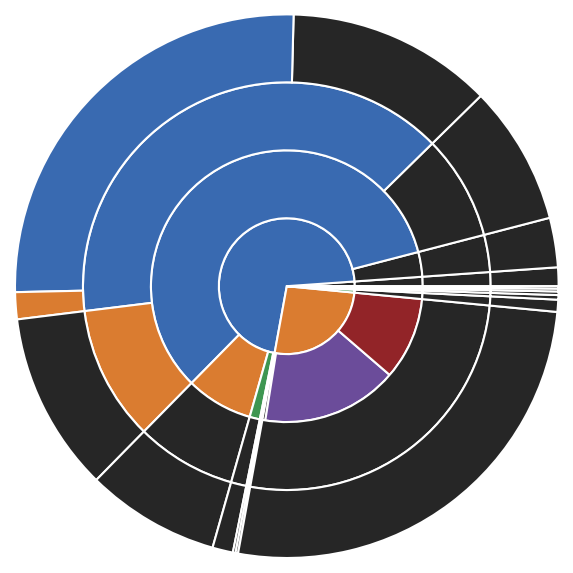
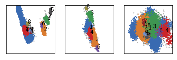
And we can finally put everything together and incorporate the child clusters into the root data set. We get an impression on how big the extracted clusters are relative to each other. In principle we have 5 or 6 dominating clusters in terms of size
[138]:
# Deep=None goes done to the bottom of the hierarchy
langerin_reduced.reel(deep=None)
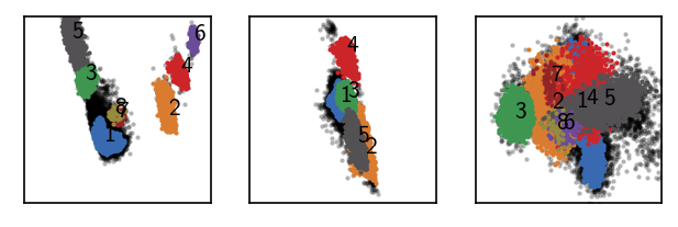
After this call, cluster labeling may not be contiguous and sorted by size, which we can fix easily.
[139]:
langerin_reduced.labels.sort_by_size()
[140]:
draw_evaluate(langerin_reduced)
[141]:
print("Label    Size")
print("=============")
print(*sorted({k: len(v) for k, v in langerin_reduced.labels.clusterdict.items()}.items()), sep="\n")
Label    Size
=============
(0, 6617)
(1, 6831)
(2, 4298)
(3, 2834)
(4, 2604)
(5, 2112)
(6, 425)
(7, 324)
(8, 191)
(9, 72)
(10, 56)
(11, 44)
(12, 42)
(13, 40)
(14, 38)
For later re-use, we save the clustering result in form of the cluster label assignments.
[148]:
# Save
np.save("md_example/cluster_labels.npy", langerin_reduced.labels)
with open("md_example/cluster_labels_info.json", "w") as f_:
    f_.write(json.dumps(langerin_reduced.labels.info.params, indent=4))
[238]:
# Read
langerin_reduced.labels = np.load("md_example/cluster_labels.npy")
with open("md_example/cluster_labels_info.json") as f_:
    langerin_reduced.labels.info = cnn.LabelInfo(None, None, json.load(f_))
We have several option to fine tune our cluster result. Depending on the used kind of validation of the result, clusters may turn out to be irelavant or splitted to much. If we want to throw out a number of clusters for any reason, we can do this by declaring all their membering points as noise:
[239]:
langerin_reduced.labels.trash([6, 7, 10, 11, 12, 13])
langerin_reduced.labels.sort_by_size()
[240]:
print("Label    Size")
print("=============")
print(*sorted({k: len(v) for k, v in langerin_reduced.labels.clusterdict.items()}.items()), sep="\n")
Label    Size
=============
(0, 7548)
(1, 6831)
(2, 4298)
(3, 2834)
(4, 2604)
(5, 2112)
(6, 191)
(7, 72)
(8, 38)
[247]:
draw_evaluate(langerin_reduced)
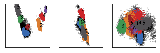
We can also group clusters together:
[248]:
langerin_reduced.labels.merge([7, 8])
langerin_reduced.labels.sort_by_size()
[249]:
draw_evaluate(langerin_reduced)
MSM estimation
Assuming our data was sampled in a time-correlated manner as it is the case for MD simulation data, we can use this clustering result as a basis for the estimation of a core-set Markov-state model.
[250]:
M = cmsm.CMSM(langerin_reduced.get_dtraj(), unit="ns", step=1)
[251]:
# Estimate csMSM for different lag times (given in steps)
lags = [1, 2, 4, 8, 15, 30]
for i in lags:
    M.cmsm(lag=i, minlenfactor=5, v=False)
    M.get_its()
[252]:
# Plot the time scales
fig, ax, *_ = M.plot_its()
fig.tight_layout(pad=0.1)
ax.set(**{
    "ylim": (0, None)
})
[252]:
[(0.0, 10459.606311240232)]
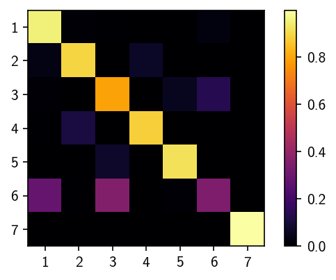
[224]:
fig, ax = plt.subplots()
matrix = ax.imshow(M.T, cmap=mpl.cm.inferno)
fig.colorbar(matrix)
ax.set(**{
    "aspect": "equal",
    "xticks": range(len(M.T)),
    "xticklabels": range(1, len(M.T) + 1),
    "yticks": range(len(M.T)),
    "yticklabels": range(1, len(M.T) + 1)
})
plt.show()
Prediction
[134]:
# Lets make sure we work on the correctly clustered object
print("Label", "r", "c", sep="\t")
print("-" * 20)
for k, v in sorted(langerin_reduced.labels.info.params.items()):
    print(k, *v, sep="\t")
Label   r       c
--------------------
1       0.19    15
2       0.4     5
3       0.25    15
4       0.4     5
5       0.375   10
6       0.375   10
7       0.19    15
8       0.19    15
9       0.5     5
10      0.5     5
11      0.5     5
12      0.5     5
13      0.375   10
14      0.375   10
15      0.5     5
16      0.19    15
17      0.25    15
[142]:
langerin_reduced_less = langerin.cut(points=(None, None, 50))
[143]:
langerin_reduced_less.calc_dist(langerin_reduced, mmap=True, mmap_file="/home/janjoswig/tmp/tmp.npy", chunksize=1000) # Distance map calculation
---------------------------------------------------------------------------
MemoryError                               Traceback (most recent call last)
<ipython-input-143-4379ad10935c> in <module>
----> 1 langerin_reduced_less.calc_dist(langerin_reduced, mmap=True, mmap_file="/home/janjoswig/tmp/tmp.npy", chunksize=1000)  # Distance map calculation

~/CNN/cnnclustering/cnn.py in calc_dist(self, other, v, method, mmap, mmap_file, chunksize, progress, **kwargs)
   1732                 len_self = self.data.points.shape[0]
   1733                 len_other = other.data.points.shape[0]
-> 1734                 self.data.distances = np.memmap(
   1735                     mmap_file,
   1736                     dtype=settings.float_precision_map[

~/CNN/cnnclustering/cnn.py in distances(self, x)
   1124     def distances(self, x):
   1125         if not isinstance(x, Distances):
-> 1126             x = Distances(x)
   1127         self._distances = x
   1128

~/CNN/cnnclustering/cnn.py in __new__(cls, d, reference)
    722             d = []
    723
--> 724         obj = np.atleast_2d(np.asarray(d, dtype=np.float_)).view(cls)
    725         obj._reference = None
    726         return obj

~/.pyenv/versions/miniconda3-4.7.12/envs/cnnclustering/lib/python3.8/site-packages/numpy/core/_asarray.py in asarray(a, dtype, order)
     81
     82     """
---> 83     return array(a, dtype, copy=False, order=order)
     84
     85

MemoryError: Unable to allocate 10.5 GiB for an array with shape (52942, 26528) and data type float64
Cluster alternatives
It is always recommended to cross validate a clustering result with the outcome of other clustering approaches. We want to have a quick look at the alternative that density-peak clustering provides.
[61]:
pydpc_clustering = pydpc.Cluster(langerin_reduced.data.points)
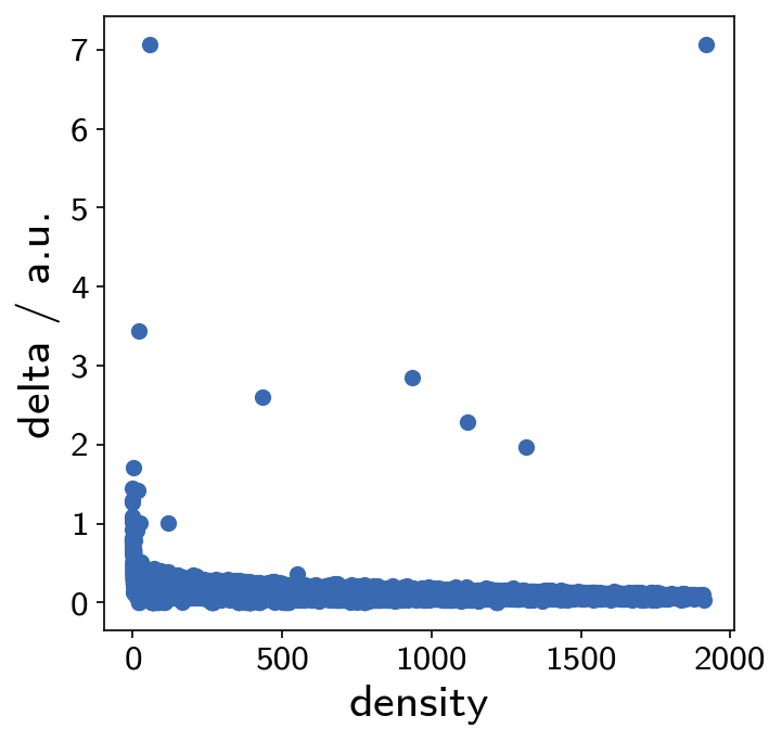
Clustering in this case is just a single step without the need of parameter specification. In the following, however, we need to extract the actual clusters by looking at the plot below. Points that are clearly isolated in this plot are highly reliable cluster centers.
[65]:
pydpc_clustering.autoplot = True
[66]:
pydpc_clustering.assign(0, 1.8)
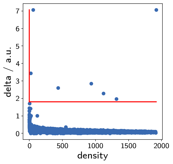
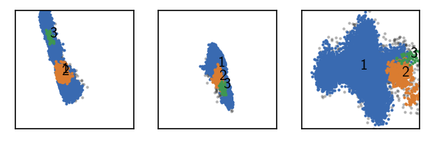
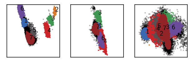
This gives us 7 clusters.
[70]:
langerin_reduced.labels = (pydpc_clustering.membership + 1)
draw_evaluate(langerin_reduced)
As we are interested in core clusters we want to apply the core/halo criterion to disregard points with low cluster membership probabilitie as noise.
[71]:
langerin_reduced.labels[pydpc_clustering.halo_idx] = 0
draw_evaluate(langerin_reduced)
[72]:
M = cmsm.CMSM(langerin_reduced.get_dtraj(), unit="ns", step=1)
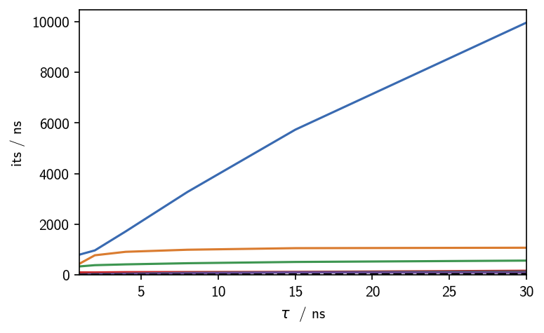
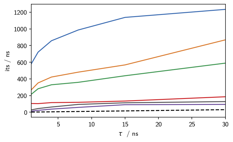
[73]:
# Estimate csMSM for different lag times (given in steps)
lags = [1, 2, 4, 8, 15, 30]
for i in lags:
    M.cmsm(lag=i, minlenfactor=5)
    M.get_its()
*********************************************************
---------------------------------------------------------
Computing coreset MSM at lagtime 1 ns
---------------------------------------------------------

Using 116 trajectories with 25900 steps over 7 coresets

All sets are connected
---------------------------------------------------------
*********************************************************


*********************************************************
---------------------------------------------------------
Computing coreset MSM at lagtime 2 ns
---------------------------------------------------------

Using 116 trajectories with 25900 steps over 7 coresets

All sets are connected
---------------------------------------------------------
*********************************************************


*********************************************************
---------------------------------------------------------
Computing coreset MSM at lagtime 4 ns
---------------------------------------------------------

Using 116 trajectories with 25900 steps over 7 coresets

All sets are connected
---------------------------------------------------------
*********************************************************


*********************************************************
---------------------------------------------------------
Computing coreset MSM at lagtime 8 ns
---------------------------------------------------------

Using 116 trajectories with 25900 steps over 7 coresets

All sets are connected
---------------------------------------------------------
*********************************************************


*********************************************************
---------------------------------------------------------
Computing coreset MSM at lagtime 15 ns
---------------------------------------------------------

Trajectories [0, 1, 73]
are shorter then step threshold (lag * minlenfactor = 75)
and will not be used to compute the MSM.

Using 113 trajectories with 25732 steps over 7 coresets

All sets are connected
---------------------------------------------------------
*********************************************************


*********************************************************
---------------------------------------------------------
Computing coreset MSM at lagtime 30 ns
---------------------------------------------------------

Trajectories [0, 1, 4, 63, 73]
are shorter then step threshold (lag * minlenfactor = 150)
and will not be used to compute the MSM.

Using 111 trajectories with 25447 steps over 7 coresets

All sets are connected
---------------------------------------------------------
*********************************************************
[74]:
# Plot the time scales
fig, ax, *_ = M.plot_its()
fig.tight_layout(pad=0.1)
[75]:
figsize = mpl.rcParams["figure.figsize"]
mpl.rcParams["figure.figsize"] = figsize[0], figsize[1] * 0.2
M.plot_eigenvectors()
mpl.rcParams["figure.figsize"] = figsize
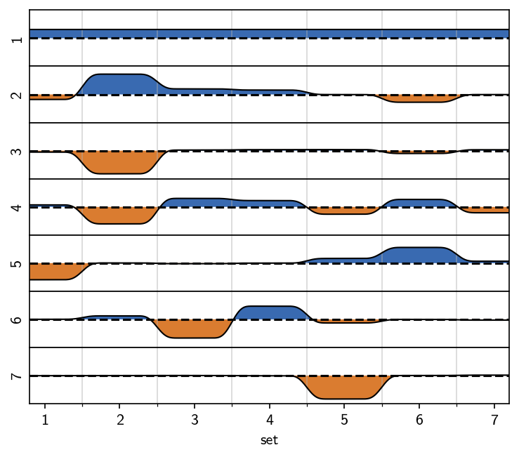
This result is in good agreement with the one we obtained manually and argualbe faster and easier to achieve. If we decide that this result is exactly what we consider valid, then this is nice. If we on the other hand want to tune the clustering result further, with respect to splitting, noise level and what is considered noise in the first place we gain more flexibility with the manual approach.